Introduction to the Excel VLOOKUP Function
The VLOOKUP function is used to look up data in a table that is organized vertically. It is applicable for both approximate and exact matching and uses wildcard characters (*, $) for partial matches.
- Syntax
=VLOOKUP (lookup_value, table_array, column_index_num, [range_lookup])
- Argument
lookup_value: The value that we need to look for in the first column of the table.
table_array: The table from which the value is extracted.
Column_index_num: That specific column from which we will retrieve a value.
- Optional Arguments
Range_lookup: TRUE means an approximate match (default). FALSE means an exact match.
Introduction to the Excel CHOOSE Function
The CHOOSE function in Excel returns a value from a list with the help of a given position or index.
- Syntax
=CHOOSE (index_num, value1, [value2], …)
- Argument
index_num: A value between 1 and 254.
value1: First chosen value
- Optional Arguments
value2: The second value to choose.
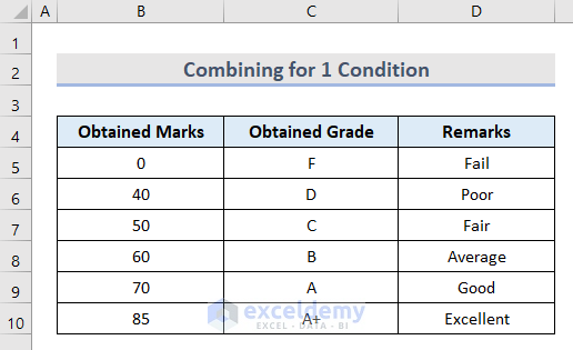
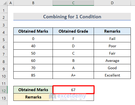
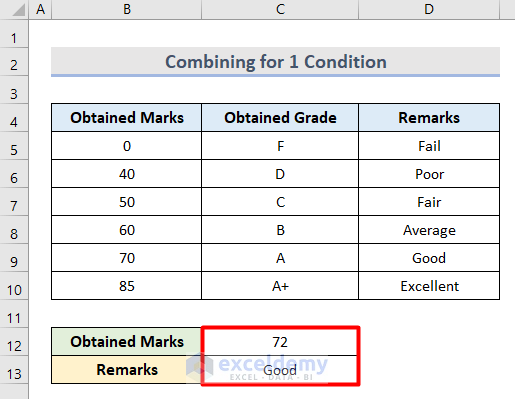
Example 1 – Combine Excel VLOOKUP & CHOOSE for a Single Condition
Suppose you have the following dataset.
- Type the condition (67 in this example) in the appropriate cell (C12).
- Insert this formula in the relevant cell (C13).
=VLOOKUP(C12,CHOOSE({1,2},B5:B10,D5:D10),2,TRUE)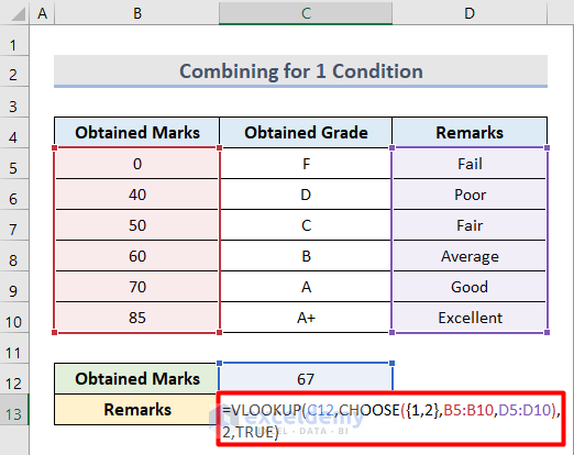
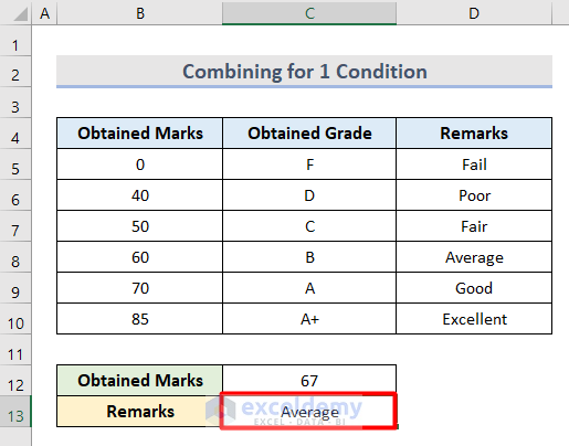
- Press Enter.
CHOOSE({1,2},B5:B10,D5:D10) is used as the table_range where {1,2} are value arguments (B5:B10,D5:D10).
The next 2 is the col_num argument for the VLOOKUP function, and TRUE is used for an approximate match.
- To prove your work, simply change the value of the condition (cell C12). The output should automatically change.
Read More: How to Use CHOOSE Function with Array in Excel
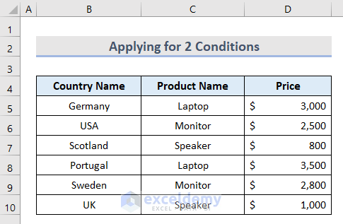
Example 2 – Apply VLOOKUP with CHOOSE for 2 Conditions
Suppose you have the following dataset.
- Add conditions to consecutive cells [(C12) and (C13) in this example].
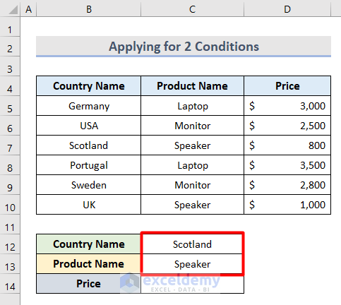
- Use this formula in the relevant cell (C14).
=VLOOKUP(C12&C13,CHOOSE({1,2},B5:B10&C5:C10,D5:D10),2,FALSE)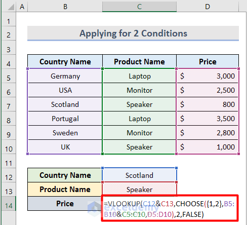
- Press Enter.
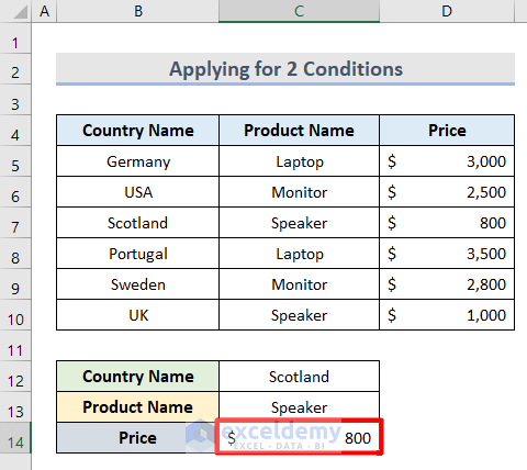
In this example, the VLOOKUP function is used to look for the values in cells C12 and C13.
CHOOSE({1,2},B5:B10&C5:C10,D5:D10) is used as the table_range where {1,2} are value arguments (B5:B10&C5:C10,D5:D10).
The next 2 is the col_num argument for the VLOOKUP function, and FALSE is used for an exact match.
Read More: How to Use CHOOSE Function to Perform IF Condition in Excel
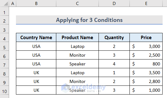
Example 3 – Insert VLOOKUP & CHOOSE for 3 Conditions
Suppose you have the following dataset.
- Add conditions to consecutive cells [(C12), (C13), and (C14)]
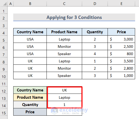
- Use this formula in the relevant cell (C15).
=VLOOKUP(C12&C13&C14,CHOOSE({1,2},B5:B10&C5:C10&D5:D10,E5:E10),2,FALSE)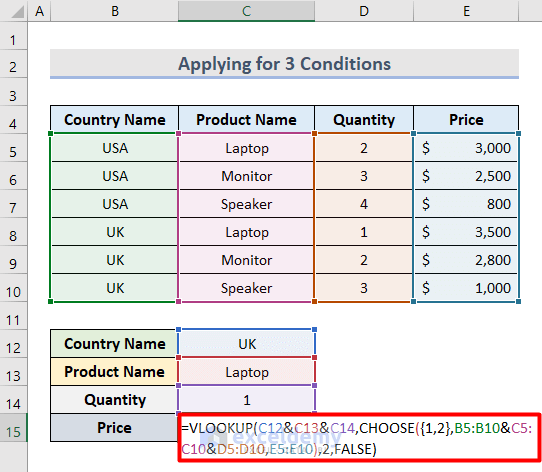
- Hit Enter.
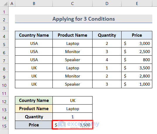
In this example, the VLOOKUP function is used to look for the value in cells C12, C13 and C14.
CHOOSE({1,2},B5:B10&C5:C10,D5:D10,E5:E10) is used as the table_range where {1,2} are value arguments (B5:B10&C5:C10&D5:D10,E5:E10).
The next 2 is the col_num argument for the VLOOKUP function and FALSE is used for an exact match.
Read More: Advanced Uses of CHOOSE Function in Excel
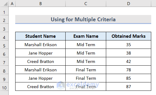
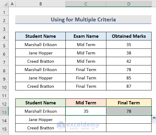
Example 4 – Excel VLOOKUP for Multiple Criteria
Suppose you have the following dataset.
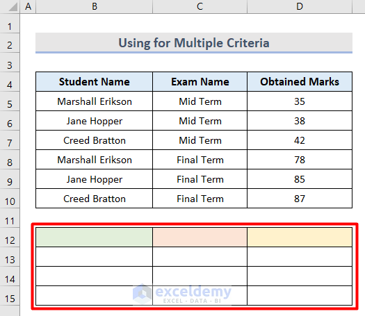
- Create a blank table (B12:D15 in this example).
- Insert the formula below in the first cell (B12).
=UNIQUE(B4:B10)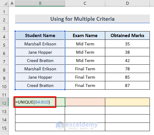
- Press Enter.
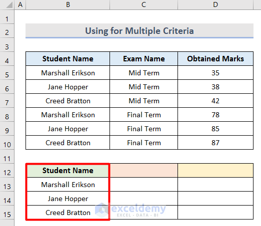
In this example, the UNIQUE function returns the unique value from the cell range B4:B10.
- Insert the following formula in the top cell in the next column (C12).
=TRANSPOSE(UNIQUE(C5:C10))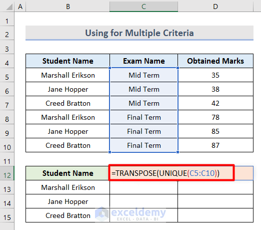
- Press Enter.
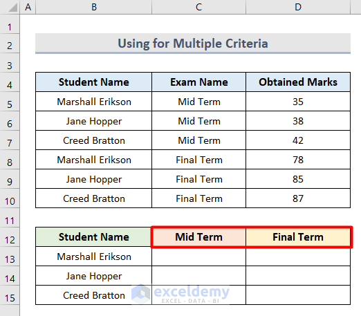
In this example, the TRANSPOSE and UNIQUE functions combined fetch and transpose unique values from the cell range C5:C10.
- Insert the following formula in the next cell (C13).
=VLOOKUP($B13&"|"&C$12,CHOOSE({1,2},$B$5:$B$10&"|"&$C$5:$C$10,$D$5:$D$10),2,0)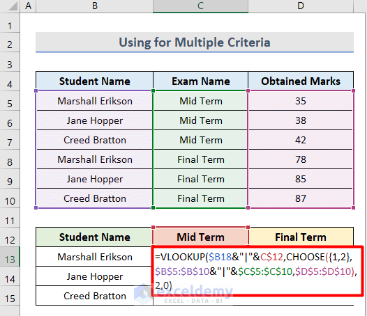
- Press Enter.
In this example, CHOOSE({1,2},$B$5:$B$10&”|”&$C$5:$C$10,$D$5:$D$10) returns a value from a range of values depending on the index number.
2 indicates the col_index_num argument.
0 represents the [range_lookup] argument.
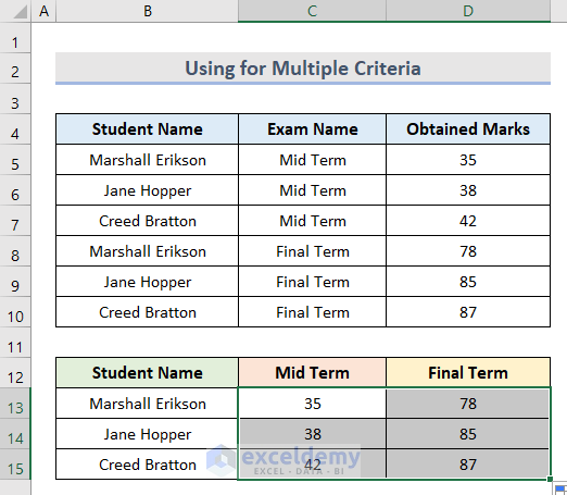
- Use the Autofill Tool to copy the formula to the remaining cells.
Example 5 – Use VLOOKUP with CHOOSE for Multiple Tables
Suppose you have the following dataset.
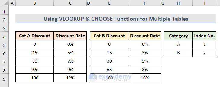
Use the VLOOKUP and CHOOSE functions to find the discount price of this dataset as shown below.
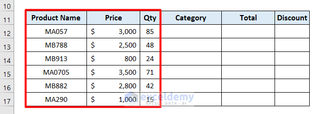
- Enter the following formula in the relevant cell (E12 in this example).
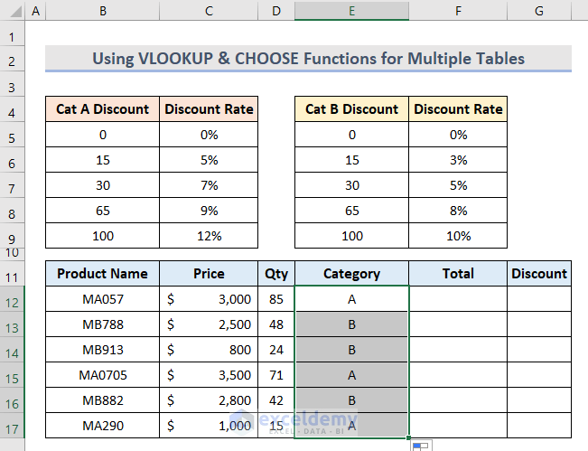
=MID(B12,2,1)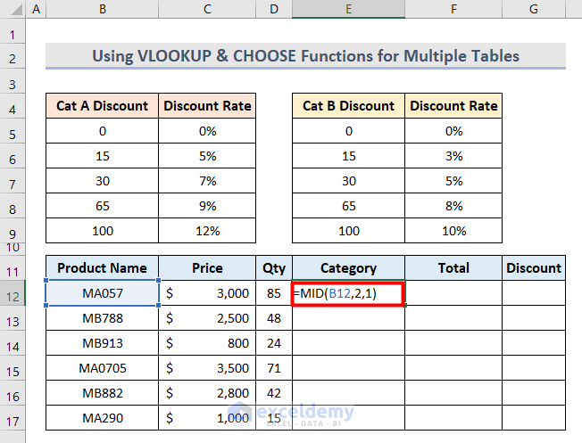
- Use the Autofill Tool to copy the formula to the remaining cells of the column.
- Put the following formula in the appropriate cell (F12) to get the total price of the first product.
=C12*D12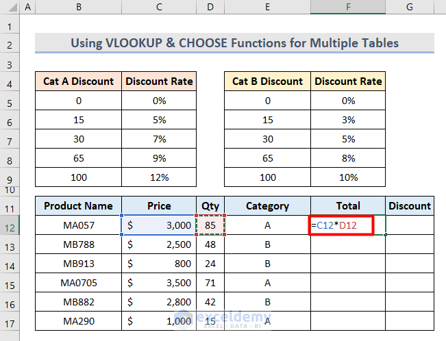
- Press Enter.
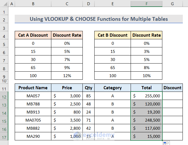
- Use the Autofill Tool to copy the formula to the remaining cells of the column.
- Select the first table (Category A cell range B4:C9).
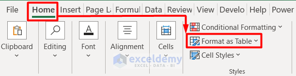
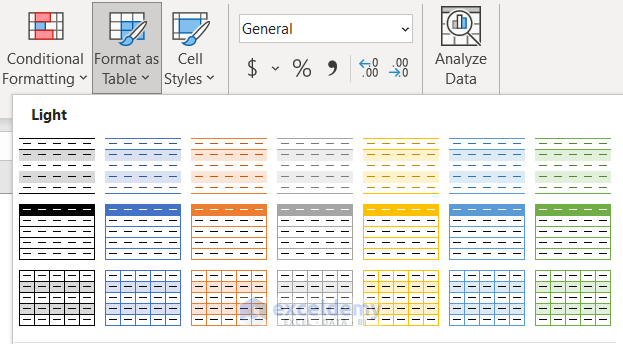
- Go to the Home tab and click on Format as Table under the Styles group.
- Select any type of table from the drop-down menu.
- Change the Table Name in the Table Design tab.

- Follow this process for the other tables as well.
- Insert the following formula in the pertinent cell (G12).
=CHOOSE(VLOOKUP(E12,Index,2,FALSE),VLOOKUP(D12,CatA,2),VLOOKUP(D12,CatB,2))*F12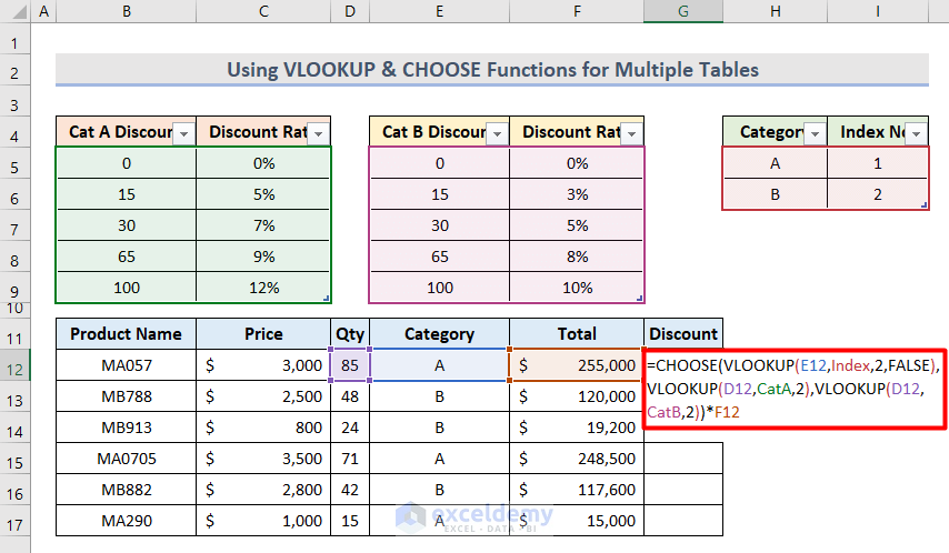
- Press Enter.
- Use the Autofill Tool to copy the formula to the remaining cells of the column.
In this example, VLOOKUP(E12,Index,2,FALSE) looks up the value in cell E12 based on the Index table with reference from column 2 in the dataset.
FALSE is for an exact match.
VLOOKUP(D12,CatA,2) and VLOOKUP(D12,CatB,2)) find the value in both category tables.
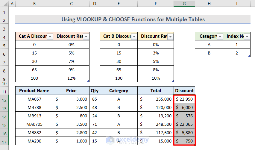
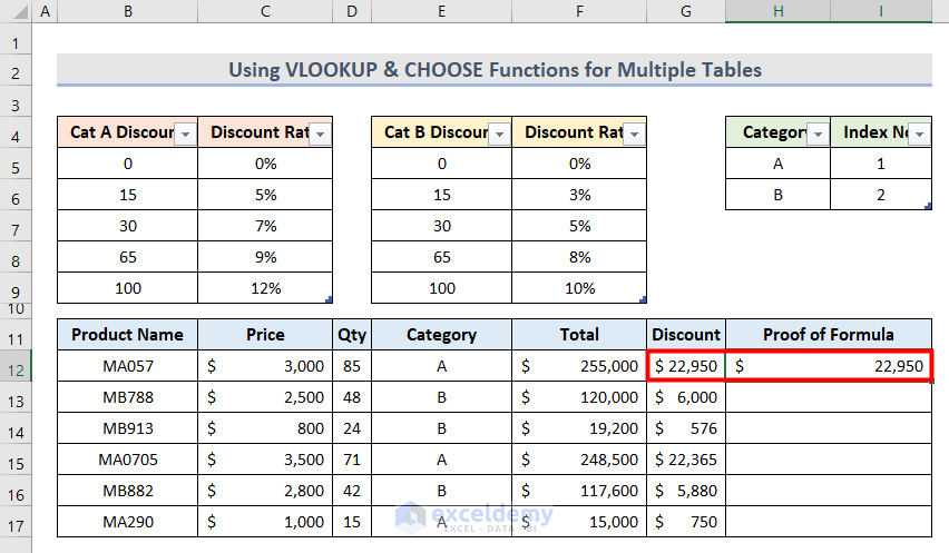
- If you want to check if the result is correct, simply multiply the total price of cell F12 by 9% according to the information in the Category A table and put this formula in cell H12.
=F12*9%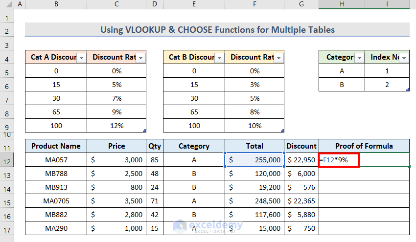
- Press Enter.
- The result should match the Discount price result from the VLOOKUP and CHOOSE functions.
Read More: How to Apply CHOOSE Function to Create Drop-Down List in Excel
Download Practice Workbook
Download this practice file and try it by yourself.
Related Articles
- How to Use CHOOSE Function in Excel for Scenarios
- How to Use Excel Formula to Choose Between Two Values
<< Go Back to Excel CHOOSE Function | Excel Functions | Learn Excel
Get FREE Advanced Excel Exercises with Solutions!

I use Excel 365. Sometimes excel hangs and it will start the undo and I cannot stop it. What causes this and how can I stop it??
Hello AARON MWALE,
Thanks for your comment. Sorry to hear that you’re facing issues with Excel.
When Excel hangs and starts an Undo action, that means Excel is trying to process a large amount of data or executing a complex operation. This may cause the program to be unresponsive for a period of time while it completes the task.
In order to stop the undo action, you can try pressing the “Esc” key on your keyboard. If this does not work, you can try pressing “Ctrl” & “Break” on your keyboard. If don’t find these helpful, you may need to wait for Excel to finish the operation before you can regain control of the program.
To prevent Excel from hanging and starting an Undo action in the future, you can try the following:
1. Limit the amount of data you are working with at one time. If you are working with a large amount of data, try breaking it up into smaller chunks that are easier for Excel to handle.
2. Close any unnecessary programs or applications running in the background. This can free up system resources and improve Excel’s performance.
3. Disable any add-ins or macros that may be causing Excel to slow down or become unresponsive.
4. Check for and install any available updates for Excel. Updates often include bug fixes and performance improvements that can help prevent Excel from hanging in the future.
5. Consider upgrading your computer hardware if it is outdated or underpowered. Excel can be resource-intensive, and having a fast and capable computer can make a big difference in its performance.
Hope you find these ways helpful to overcome your issues.
Regards,
Rafi
ExcelDemy team