Introduction to Excel CHOOSE Function
- The CHOOSE function requires two arguments: index_num and value1, along with optional additional values.
- index_num represents the position number of the values (e.g., 1 for value1, 2 for value2, and so on).
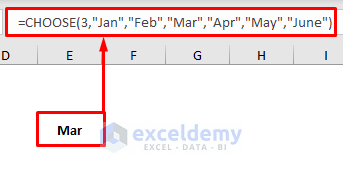
- For instance, if you enter =CHOOSE(3,”Jan”,”Feb”,”Mar”,”Apr”,”May”,”June”) in a cell, the output will be Mar because it corresponds to the third value in the specified list.
Syntax:
CHOOSE(index_num, value1, [value2]….)
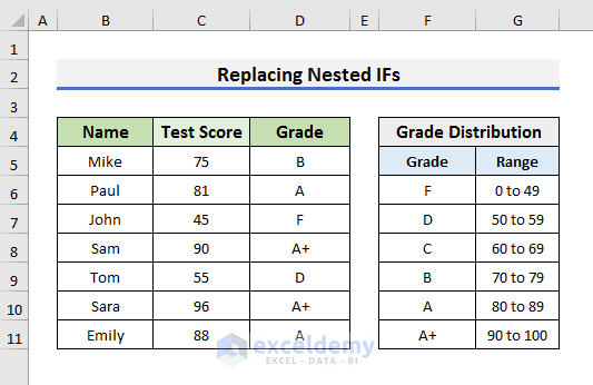
Application 1 – Replace Nested IFs
Nested IFs can become complex and unwieldy. The CHOOSE function provides an elegant alternative.
1.1 Return Value Based on Conditions
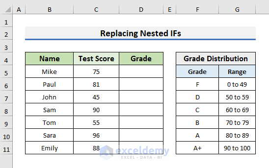
Suppose we have a dataset of test scores for students, and we want to assign grades based on certain conditions.
Instead of nested IFs, we can use the CHOOSE function. Here’s how:
- Let’s say the test score is in cell C5.
- The formula to assign grades would be:
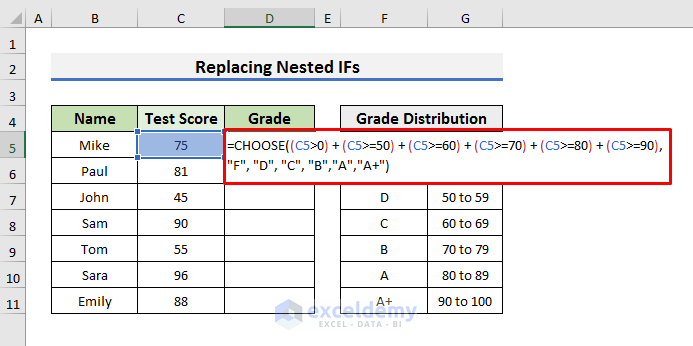
=CHOOSE((C5>0)+(C5>=50)+(C5>=60)+(C5>=70)+(C5>=80)+(C5>=90),"F","D","C","B","A","A+")
How Does the Formula Work?
- (C5>0)+(C5>=50)+(C5>=60)+(C5>=70)+(C5>=80)+(C5>=90): In this part of the formula, we have used the Grade Distribution as the index number inside the CHOOSE function. As there are multiple index numbers based on the situation, we have used the plus (+) operator to make an OR operation.
- “F”,”D”,”C”,”B”,”A”,”A+”: This part contains the values corresponding to the index numbers. Depending on the index number, the CHOOSE function will return the grades. For example, if the matched index number is between 80 to 89, then it will print “A”.
- Press Enter and drag the Fill Handle down.
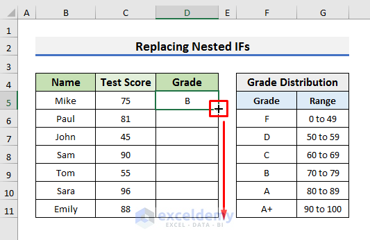
- You will be able to assign the grades based on the test scores.
1.2 Calculations Based on Criteria
Let’s consider a dataset with sales amounts for sellers and corresponding commission percentages. We want to find the commission amount for each seller based on their sales range.
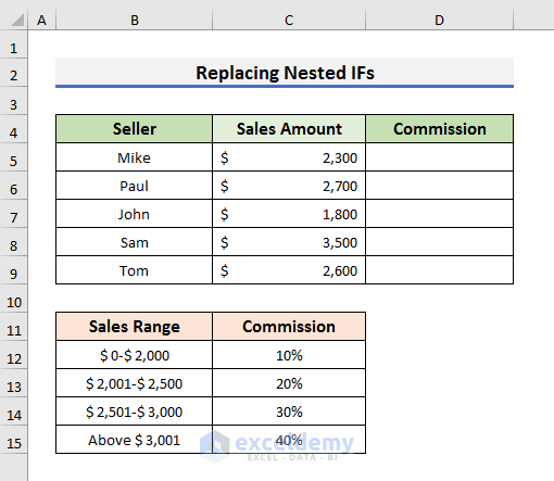
STEPS:
- Select cell D5 and enter the formula below:
=CHOOSE((C5>=0)+(C5>=2001)+(C5>=2501)+(C5>=3001),C5*0.1,C5*0.2,C5*0.3,C5*0.4)-
- Explanation:
- The index number determines the sales range (e.g., 0-2000, 2001-2500, etc.).
- The CHOOSE function multiplies the sales amount (in cell C5) by the corresponding commission percentage.
- The result is the commission for each seller.
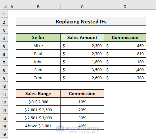
- Explanation:

This formula is similar to the previous one. But it multiplies the value of Cell C5 with the Commission percentage based on the index number and then returns the result.
- Press Enter and drag down the Fill Handle to see the commission for each seller.
Read More: How to Use CHOOSE Function to Perform IF Condition in Excel
Application 2 – Apply CHOOSE Function for Left VLOOKUP in Excel
Let’s explore how to use the CHOOSE function in conjunction with VLOOKUP for left-sided lookups in Excel. When dealing with multiple criteria, the standard VLOOKUP may not suffice. However, by combining the CHOOSE function with VLOOKUP, we can extract specific values based on various conditions. Here are the non-array and array formulas for achieving this:
To explain both formulas, we will use a dataset that contains the First Name and Last Name of some employees. We will extract the Department based on the names.
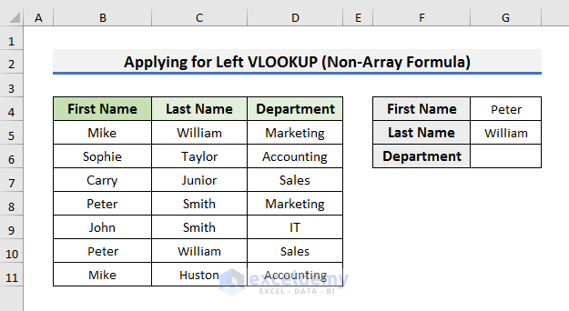
2.1 Non-Array Formula
- To create a non-array formula, we’ll use a helper column alongside the VLOOKUP and CHOOSE functions.
- Follow these steps:
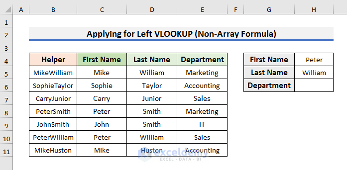
- Insert a helper column (e.g., Column B) on the left side of your data.
- Concatenate the First Name and Last Name in the helper column. For example, in cell B5, enter the formula:
=C5&D5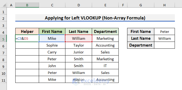
-
- Press Enter and drag the Fill Handle down.
-
- In Cell H6 enter the following formula:
=VLOOKUP($H$4&$H$5,CHOOSE({1,2},$B$5:$B$11,$E$5:$E$11),2,FALSE)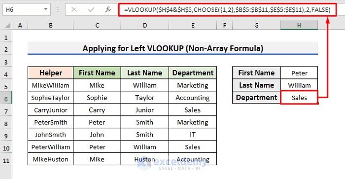
Here,
-
-
- The CHOOSE function creates a lookup table with Columns B & C.
- The VLOOKUP function searches for the PeterWilliam value in Column B and returns the corresponding value from the lookup table that the CHOOSE function creates.
-
Read More: How to Use VLOOKUP with CHOOSE Function in Excel
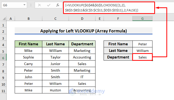
2.2 Array Formula
If we avoid using a helper column, the formula becomes an array formula.
- In cell G6, enter the following formula:
=VLOOKUP($G$4&$G$5,CHOOSE({1,2},$B$5:$B$11&$C$5:$C$11,$D$5:$D$11),2,FALSE)- Press Ctrl + Shift + Enter to evaluate it.
-
- This array formula looks for the concatenated value of cell G4 and Cell G5 in the lookup table.
- This time the CHOOSE function creates a lookup table of two columns. The first column concatenates the value of the range B5:B11 and C5:C11 and the second column stores the Department names.
- Depending on the First and Last names, it returns the Department name.
Read More: How to Use CHOOSE Function with Array in Excel
Application 3 – Using CHOOSE for Sum of Selected Variables
We can also apply the CHOOSE function inside the SUM function to dynamically find the total sales for a specific month. Consider a dataset with sales amounts for the first three months.
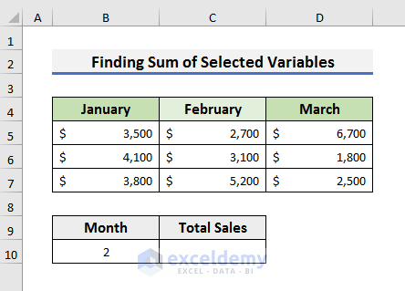
- Select Cell C10 and enter the formula below:
=SUM(CHOOSE(B10,B5:B7,C5:C7,D5:D7))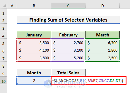
In this formula:
-
-
- The CHOOSE function selects the range based on the month number that we insert in cell B10. If we enter 2 in cell B10, then the formula becomes:
-
=SUM(CHOOSE(2,B5:B7,C5:C7,D5:D7))
-
-
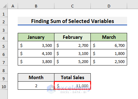
- The CHOOSE function returns the range C5:C7 based on the index number.
- The formula acts as:
-
=SUM(C5:C7)
That is how we get the total sales for the selected month.
- Press Enter to see the total sales for February.
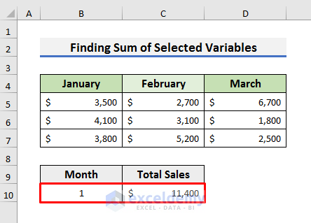
- To see the total sales for January, enter 1 in Cell B10.
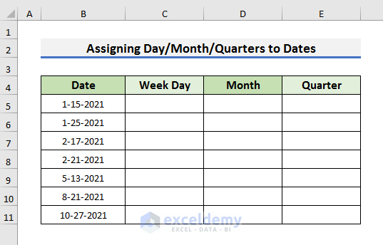
Application 4 – Assigning Weekdays, Months, and Quarters to Dates
Assigning day/month/quarters to dates is another feature of the CHOOSE function. The help of the WEEKDAY function is required. The dataset below contains some dates. Let’s extract the Week Day, Month, and Fiscal Quarters for the dates.
- To assign weekdays to dates, enter the following formula in cell C5:
=CHOOSE(WEEKDAY(B5),"Sun","Mon","Tue","Wed","Thu","Fri","Sat")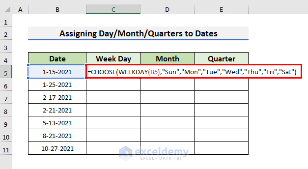
The WEEKDAY function returns the index number for the CHOOSE function, which corresponds to the day of the week.
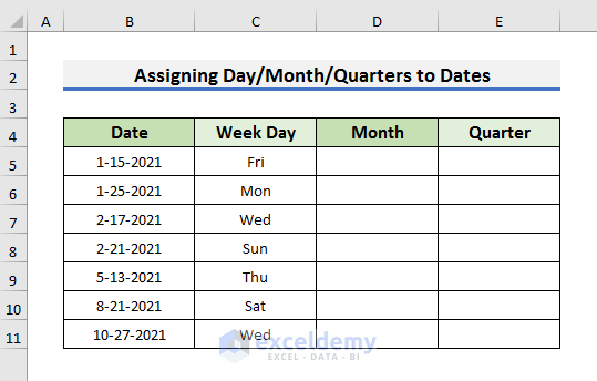
- Press Enter and drag the Fill Handle down to see weekdays for all dates.
- To assign months to dates, enter the following formula in Cell D6:
=CHOOSE(MONTH(B5), "Jan","Feb","Mar","Apr","May","Jun","Jul","Aug","Sep","Oct","Nov","Dec")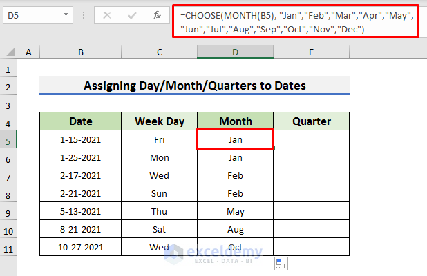
- The MONTH function finds the month number and uses it as the index number.
- For fiscal quarters, enter the following formula in cell E5:
=CHOOSE(MONTH(B5), 3,3,3,4,4,4,1,1,1,2,2,2)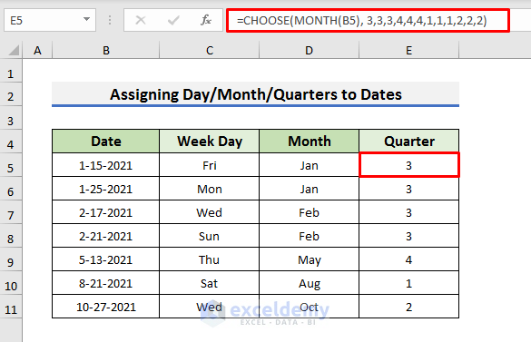
This assigns the appropriate quarter based on the month.
Application 5 – Using CHOOSE Function to Return Value Based on Index Number
In this basic application, we return a value from a list based on an index number. Suppose we have employees with index numbers.
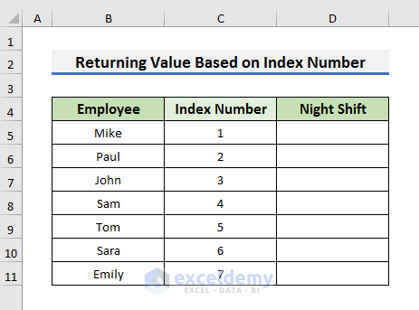
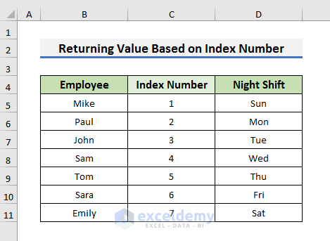
- To assign weekdays for night shifts, enter the following formula in cell D5:
=CHOOSE(C5,"Sun","Mon","Tue","Wed","Thu","Fri","Sat")
- Cell C5 contains the index number, and the CHOOSE function returns the corresponding weekday.
- Press Enter and drag the Fill Handle down.
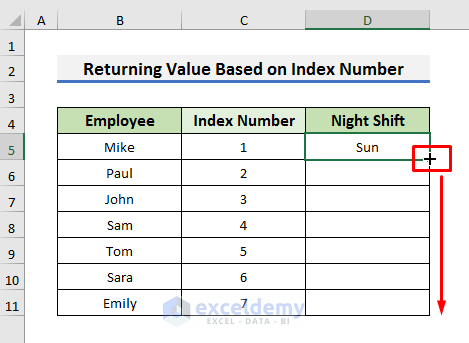
- You will be able to return a value based on the index number.
Application 6 – Apply CHOOSE Function for Reverse VLOOKUP in Excel
The reverse VLOOKUP allows us to search for a value in other columns. Given a dataset with Last Name, First Name, and Department, we want to find the First Name and Department based on the Last Name.
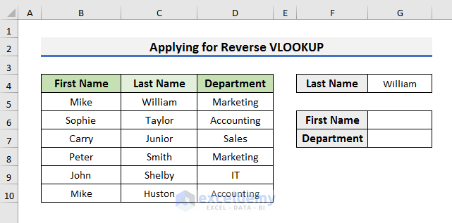
- To get the First Name, select Cell G6 and enter the formula below:
=VLOOKUP($G$4,CHOOSE({1,2,3},$C$5:$C$10,$B$5:$B$10,$D$5:$D$10),2,FALSE)- Press Enter to see the result.
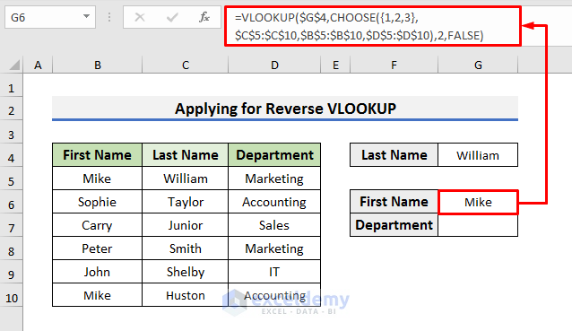
- The CHOOSE function creates a new table with Last Name, First Name, and Department columns.
- The VLOOKUP formula looks for the value in cell G4 and returns the corresponding First Name.
- Enter the formula below in cell G7 to get the Department of the employee:
=VLOOKUP($G$4,CHOOSE({1,2,3},$C$5:$C$10,$B$5:$B$10,$D$5:$D$10),3,FALSE)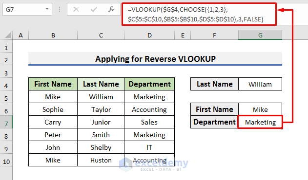
- This retrieves the Department based on the Last Name.
Application 7 – Generate Random Data Using CHOOSE Function
Suppose we want to randomly assign groups to employees for different tasks. For that purpose, we can use the RANDBETWEEN function. The RANDBETWEEN function returns a series of numbers from the specified range of numbers.
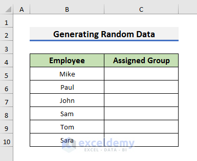
- To achieve this, enter the following formula in cell C5:
=CHOOSE(RANDBETWEEN(1,3),"G-1","G-2","G-3")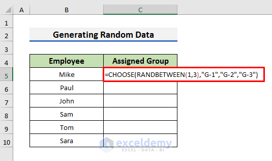
- The RANDBETWEEN function generates a random number (1, 2, or 3), which serves as the index for the CHOOSE function.
- Based on the index, the CHOOSE function selects a group from the list.
- Press Enter and drag down the Fill Handle to copy the formula down to Cell C10.
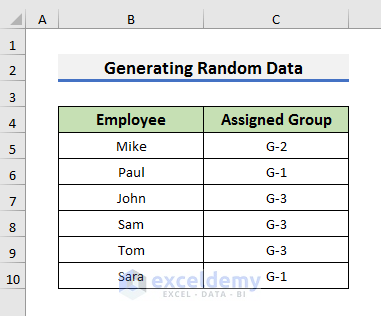
Note: The RANDBETWEEN function is a volatile function. If you make any changes to the sheet, the assigned groups will automatically change. To make the assigned groups hard-coded, you can paste the values after obtaining the groups.
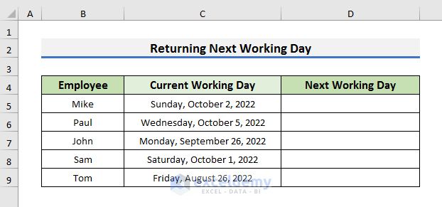
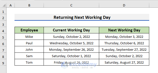
Application 8 – Return Next Working Day Using CHOOSE Function
Let’s find the next working day based on the current working day. We will find the next working day using the WEEKDAY function with the CHOOSE function.
- In cell D5, enter this formula:
=C5+CHOOSE(WEEKDAY(TODAY()),1,1,1,1,1,3,2)- Press Enter.
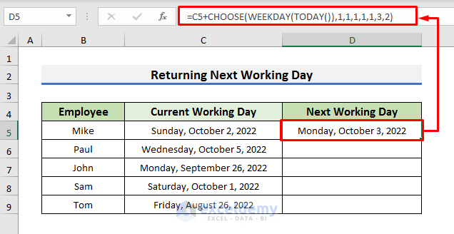
- The WEEKDAY function returns the index number for today’s date (1 for Sunday, 2 for Monday, etc.).
- The CHOOSE function selects a value (1, 3, or 2) based on the index.
- Add this value to the current date (in cell C5) to get the next working day.
- Drag the Fill Handle down to copy the formula.
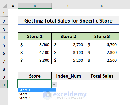
Application 9 – Get Total Sales for Specific Store Using CHOOSE Function
Imagine we have sales data for different stores, and we want to calculate the total sales for a specific store selected from a drop-down list.
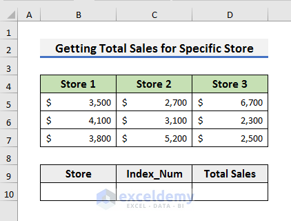
- Select cell B10.
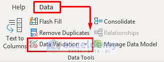
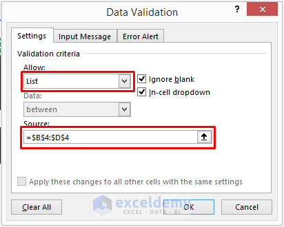
- Go to the Data tab and select Data Validation. It will open the Data Validation box.
- Select List in the Allow field.
- Enable editing in the Source field and select the range B4:B7.
- Click OK to proceed.
- A drop-down list has been created.
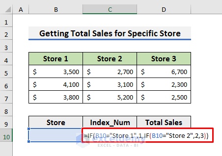
- In cell C10, enter this formula to assign index numbers to each store:
=IF(B10="Store 1",1,IF(B10="Store 2",2,3))-
- If B10 contains Store 1, it returns 1; if Store 2, it returns 2; otherwise, it returns 3.
- Press Enter.
- Select cell D10 and calculate the total sales using:
=SUM(CHOOSE(C10,B5:B7,C5:C7,D5:D7))- Press Enter.
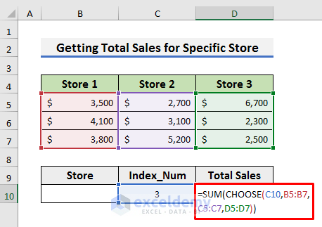
The CHOOSE function selects the appropriate range (sales data) based on the index.
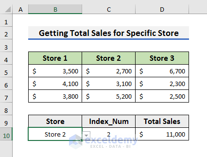
- Adjust the drop-down selection to see the total sales for the chosen store.
Read More: How to Apply CHOOSE Function to Create Drop-Down List in Excel
Download Practice Workbook
You can download the practice workbook from here:
Related Articles
- How to Use Excel Formula to Choose Between Two Values
- How to Use CHOOSE Function in Excel for Scenarios
<< Go Back to Excel CHOOSE Function | Excel Functions | Learn Excel
Get FREE Advanced Excel Exercises with Solutions!
