A drop-down list is a feature in Microsoft Excel that allows one to create a list of items to select from. This can be helpful when we have a list of items that we need to choose from, and we don’t want to have to type them all out. In this article, I will try to explain 3 simple ways to create a drop-down list with the CHOOSE function in Excel. I hope it will be very helpful for you if you are looking for a way to create a drop-down list with the CHOOSE Function in Excel.
Creating Drop-Down List Using CHOOSE Function in Excel: 3 Simple Ways
1. Apply CHOOSE Function to Create a Dependent Drop-Down List
We can create a drop-down list with a specific formula for some specific values. In order to create a dependent drop-down list, we can use the CHOOSE function. The whole procedure is described in the following section.
Steps:
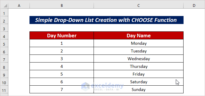
- First of all, create an organized dataset. For me, I have created a dataset of weekdays with a specific number in Day Number and Day Name columns.
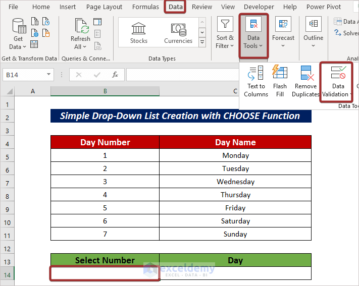
- Now, select a cell (i.e. B14) to create a drop-down list.
- Next, go to the Data tab.
- From the ribbon, click on Data Tools.
- After that, pick the Data Validation option.
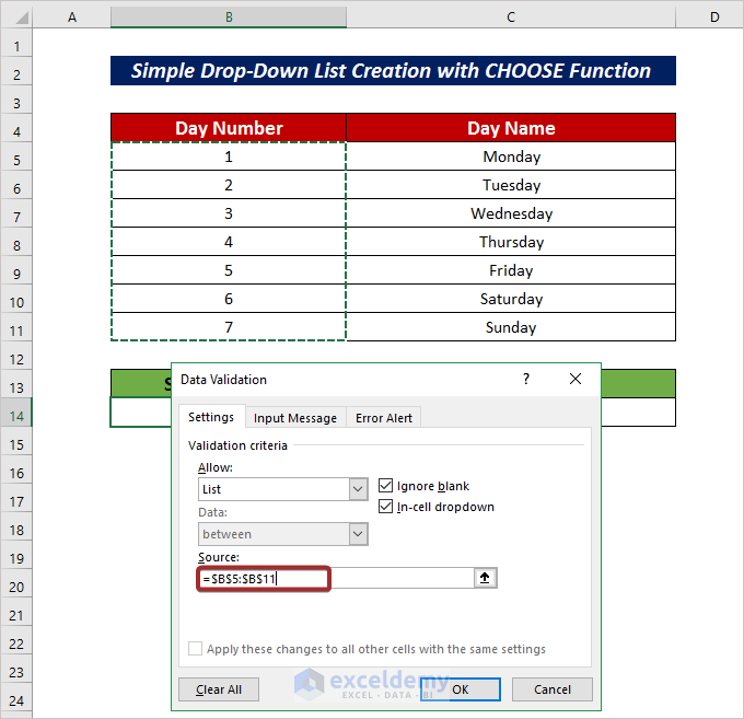
- Pick List from the Allow section from the Data Validation wizard.

- Set range (i.e. $B$5:$B$11) in the Source section.
- Then, press OK.
Thus, we can have a drop-down list on the defined cell.
- Next, pick a cell and apply the following formula where you want to have the result based on the drop-down selection.
=CHOOSE(B14,C5,C6,C7,C8,C9,C10,C11)Here, the CHOOSE function returns the output based on the index number that is mentioned by B14.
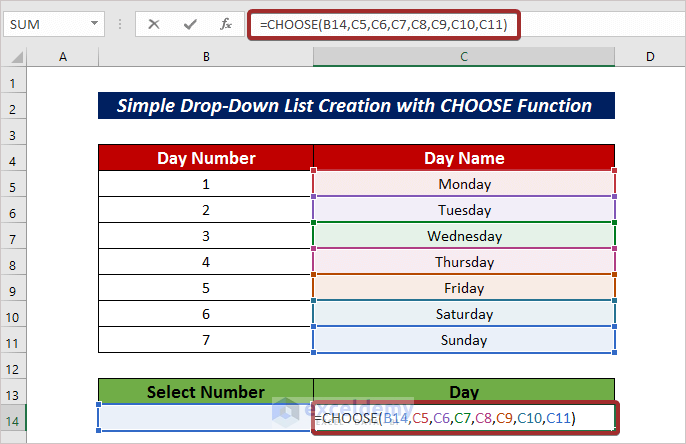
- Finally, press the ENTER button and choose any option from the drop-down list to have the related result.
Read More: How to Use CHOOSE Function to Perform IF Condition in Excel
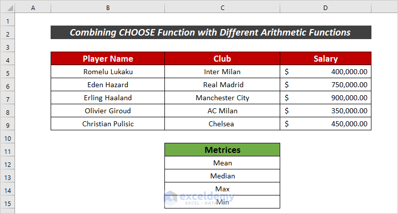
2. Combine CHOOSE Function with Different Arithmetic Functions to Create a Drop-Down List
We can also assign different arithmetic functions with the CHOOSE function to have results from the drop-down list. It’s not a difficult task to do. You will agree with me after reading the whole procedure listed below.
Steps:
- Create an organized dataset as a first step. Here, I have arranged the salary of different footballers in Player Name, Club, and Salary I have also mentioned the particulars that I want to add in the drop-down list in the Matrices column.
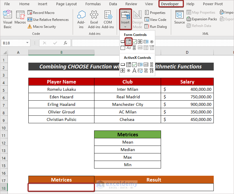
- Afterward, pick a cell (i.e. B18) to create a drop-down list.
- Next, go to the Developer tab.
- From the ribbon, click on Insert.
- After that, pick the Combo Box (Form Control).
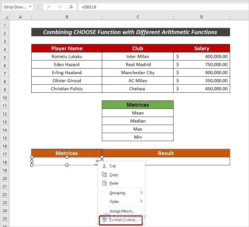
The drop-down box will be in the selected cell.
- Now, right-click on the mouse and select the Format Control… option.
- Go to Control and assign the Input range (i.e. $C$12:$C$15) and Cell Link (i.e. $B$18).
- Then, click on OK.

- Followingly, select a cell (i.e. C18) and apply the following formula where you want to have the result based on the drop-down selection.
=CHOOSE(B18,AVERAGE(D5:D9),MEDIAN(D5:D9),MAX(D5:D9),MIN(D5:D9))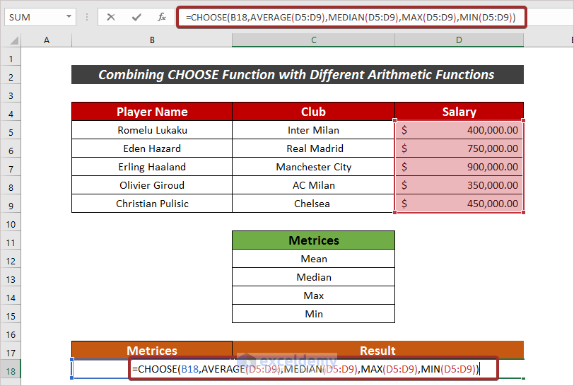
- Finally, you can have your desired result just by selecting it from the drop-down list.
3. Merge CHOOSE and MATCH Functions to Create a Drop-Down List
The creation of a calculator merging the CHOOSE and MATCH functions is also possible. We can add a drop-down box with different operation names. The procedure is described in the following section.
Steps:
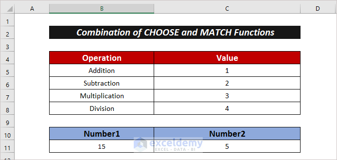
- As a first step, organize your data properly. I have set the operations name along with a number in the Operation and Value columns, I have also added two numbers in the dataset with which I will apply the operators.
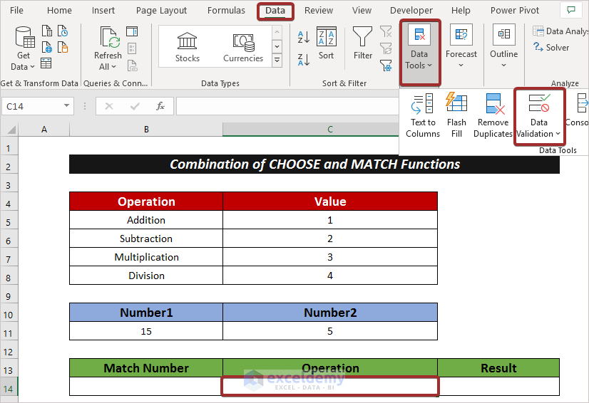
- Now, select a cell (i.e. C14) to create a drop-down list.
- Next, go to the Data tab.
- From the ribbon, click on Data Tools.
- After that, pick the Data Validation option.
- After that, pick List from the Allow section and set the range (i.e. $B$5:$B$11) in the Source section.
- Press OK to finish the drop-down list creation process.

Thus, we can have operation names in a drop-down list.

- Now, input the following formula with the MATCH function in your preferred cell (i.e. B14) to have the match number of the operation.
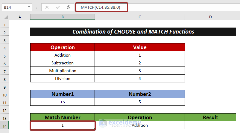
=MATCH(C14,B5:B8,0)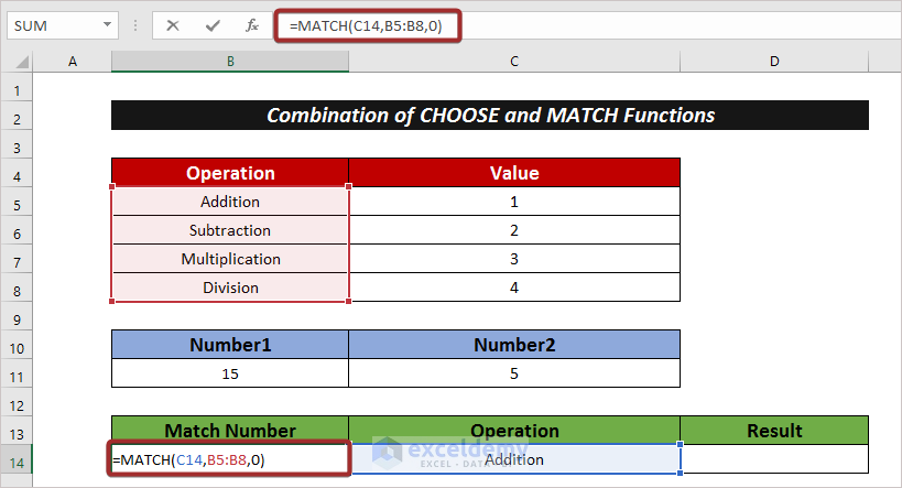
- Press the ENTER button to have the match number.
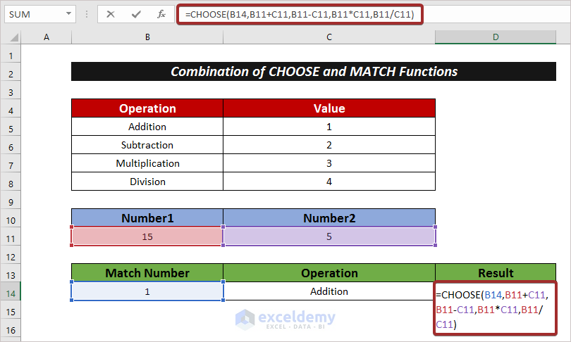
- Along with that, pick a cell (i.e. D14) and apply the following formula where you want to have the result based on the drop-down selection.
=CHOOSE(B14,B11+C11,B11-C11,B11*C11,B11/C11)
- Finally, hit ENTER to finish the process.
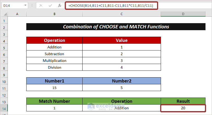
Thus, we can create a drop-down list with the CHOOSE and MATCH functions.
Read More: Advanced Uses of CHOOSE Function in Excel
Download Practice Workbook
Conclusion
That’s all for this article. In this article, I have tried to explain 3 simple ways to create a drop-down list with the CHOOSE function in Excel. It will be a matter of great pleasure for me if this article could help any Excel user even a little. For any further queries, comment below. You can visit our site for more articles about using Excel.
Related Articles
- How to Use CHOOSE Function with Array in Excel
- Use RANDBETWEEN with CHOOSE Function in Excel
- How to Use CHOOSE Function in Excel for Scenarios
- Use VLOOKUP with CHOOSE Function in Excel
- How to Use Excel Formula to Choose Between Two Values
<< Go Back to Excel CHOOSE Function | Excel Functions | Learn Excel
Get FREE Advanced Excel Exercises with Solutions!
