
If you’ve ever built a drop-down list in Excel using Data Validation, you’ve probably run into this annoying problem: you add a new item to your source list, but it doesn’t show up in the drop-down. You must go back, edit the named range or the validation source, and manually extend it. A dynamic drop-down list fixes this permanently. A dynamic drop-down list automatically expands or refreshes its options when you add, remove, or change items in the source data. This is extremely useful for data entry forms, dashboards, and reports in Excel. No more manually updating ranges.
In this tutorial, we will show how to build a dynamic drop-down list that updates itself. Add a new item to your source list, and it instantly appears as an option in the drop-down.
Method 1: The Excel Table Trick (Easiest)
This is the simplest and most reliable method, and it works in Excel 2010 and later.
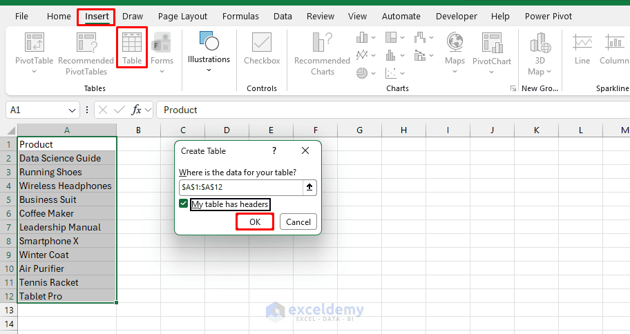
Step 1: Turn Your Source List into a Table
- Type your list of items in a column
- Give it a header like “Product”
- Select the range
- Go to the Insert tab >> select Table or press Ctrl + T
- Make sure “My table has headers” is checked
- Click OK
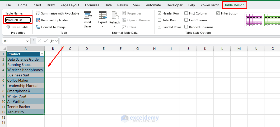
- Excel will auto-name it something like Table1
- Go to the Table Design tab >> under Table Name, name it ProductList
Step 2: Create the Drop-Down Using the Table Column
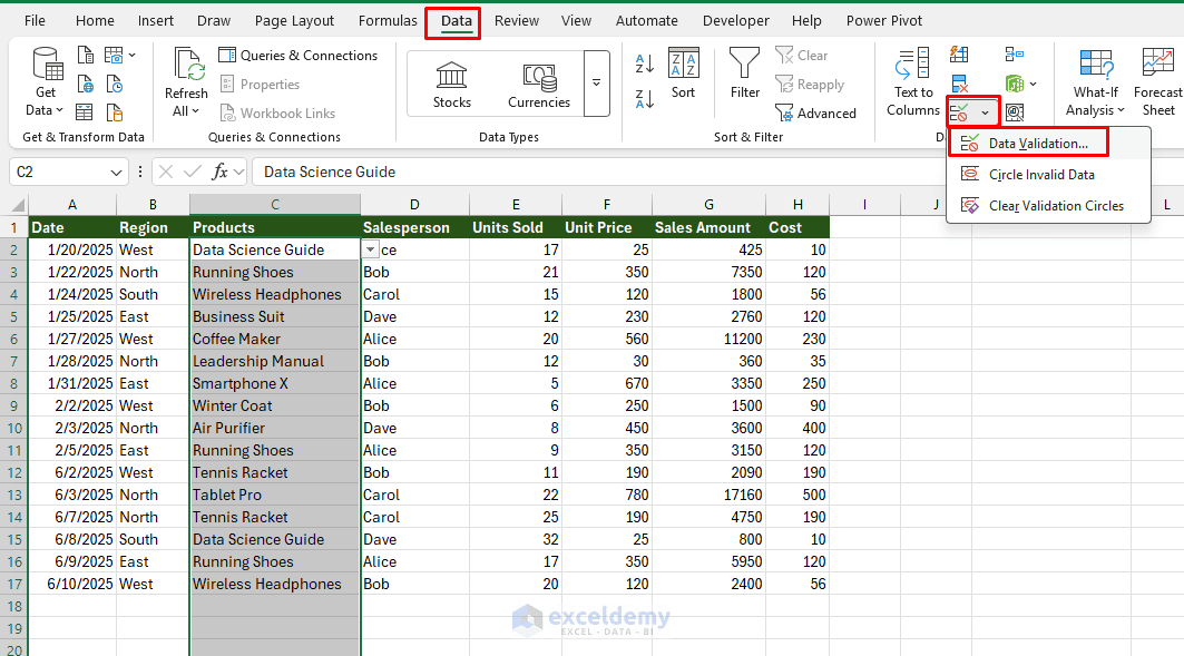
- Click on the cell where you want your drop-down
- Go to the Data tab >> select Data Validation
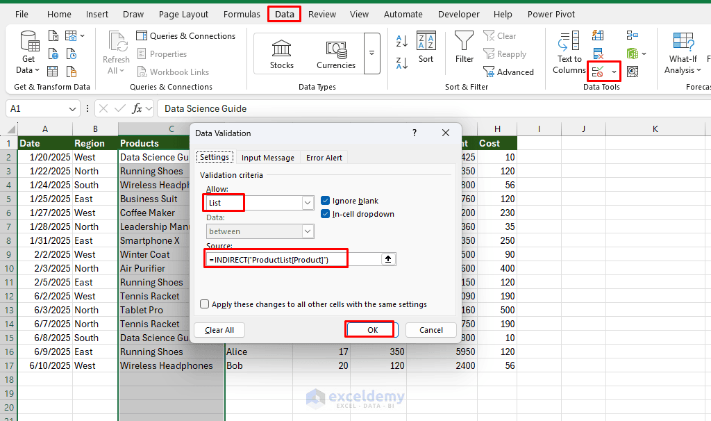
- Under Allow, choose List
- In the Source box, type:
=INDIRECT("ProductList[Product]")
This converts the text reference into the Product column of the Excel table named ProductList. It is commonly used as a dynamic Data Validation source.
- Click OK
Verify & Test:
- Go back to your table and type a new product in the row right below the last entry
- Excel will auto-expand the table
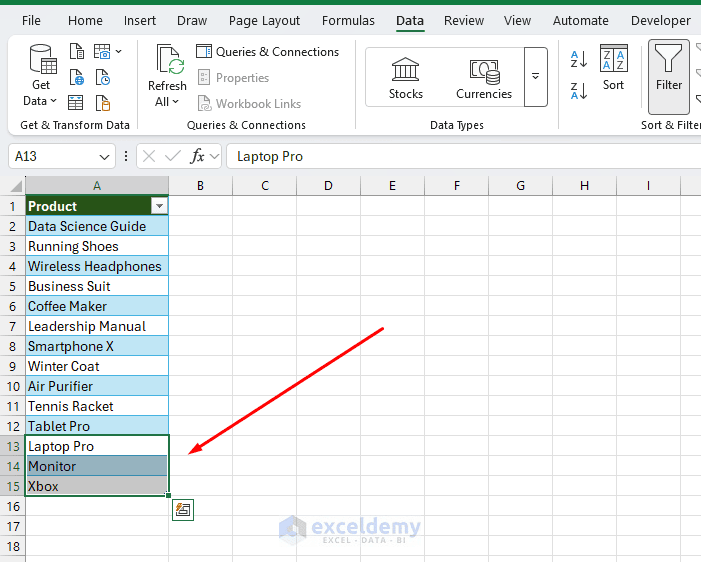
- Click your drop-down cell, and the new item is already there
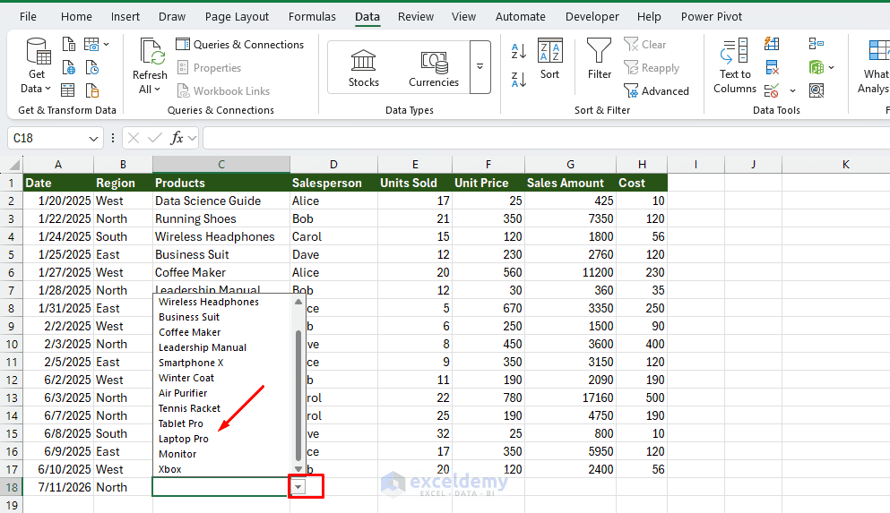
Why this works: Structured references such as Table[Column] automatically resize as rows are added or removed. The drop-down source grows with the table — no formulas needed.
Method 2: UNIQUE + SORT (Best for Excel 365)
Use this when your data contains duplicates or isn’t already clean, and you want the drop-down to automatically show a sorted, deduplicated list.
Step 1: Set Up a Spill Formula
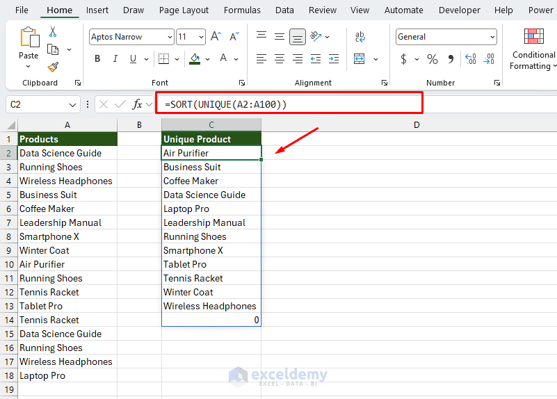
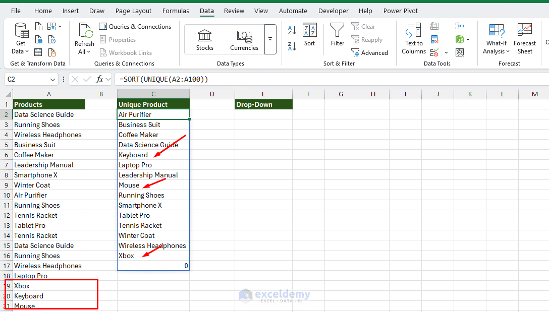
Suppose your raw data has duplicate values. To create a drop-down, use:
=SORT(UNIQUE(A2:A100))
This creates a “spill range” — a dynamically sized list of unique, sorted values.
Step 2: Reference the Spill Range in Data Validation
- Select your drop-down cell
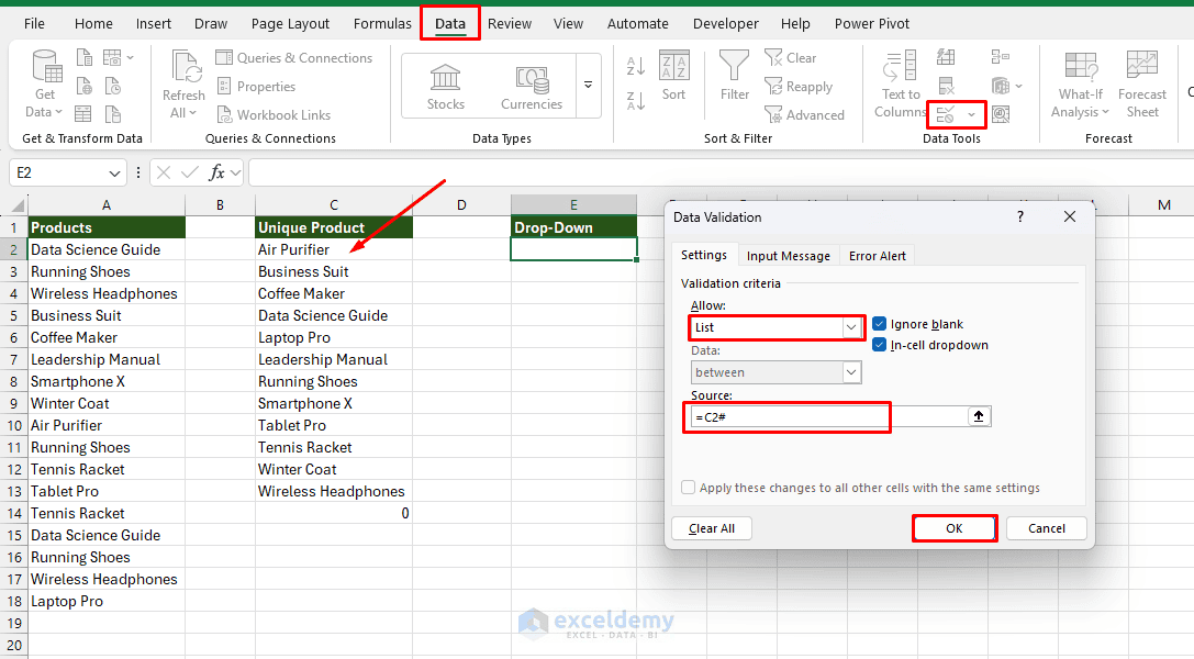
- Go to the Data tab >> select Data Validation >> select List
- In “Source,” type:
=C2#
The # symbol is the spill range operator; it tells Excel to use whatever range this formula spills into, however large it gets.
- Click OK
Test It:
- Add a new (even duplicate) value to your raw data column
- The UNIQUE formula recalculates instantly, and the spill range grows automatically
- The drop-down updates automatically
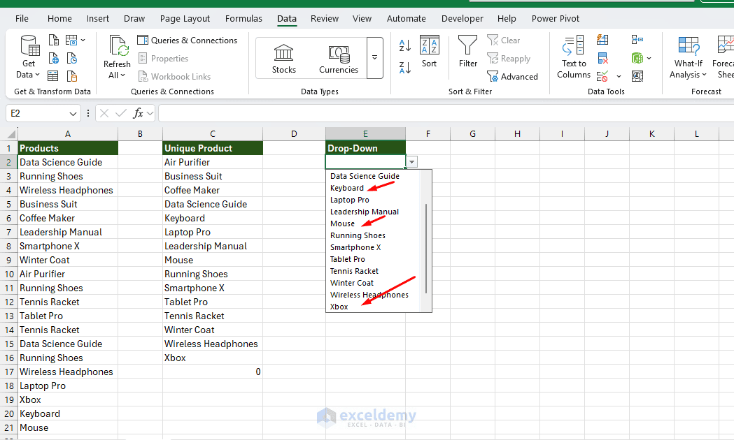
Bonus: Filter Out Blanks
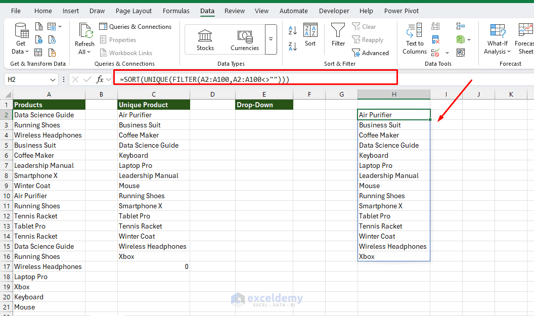
If your source range has empty cells, wrap the formula like this to avoid a blank item appearing in your drop-down:
=SORT(UNIQUE(FILTER(A2:A100,A2:A100<>"")))
Method 3: Named Range with OFFSET or INDEX (Works in Any Excel Version)
If you’re on an older Excel version without tables or dynamic arrays, use a named range built with a formula that auto-expands.
Step 1: Create the Named Range
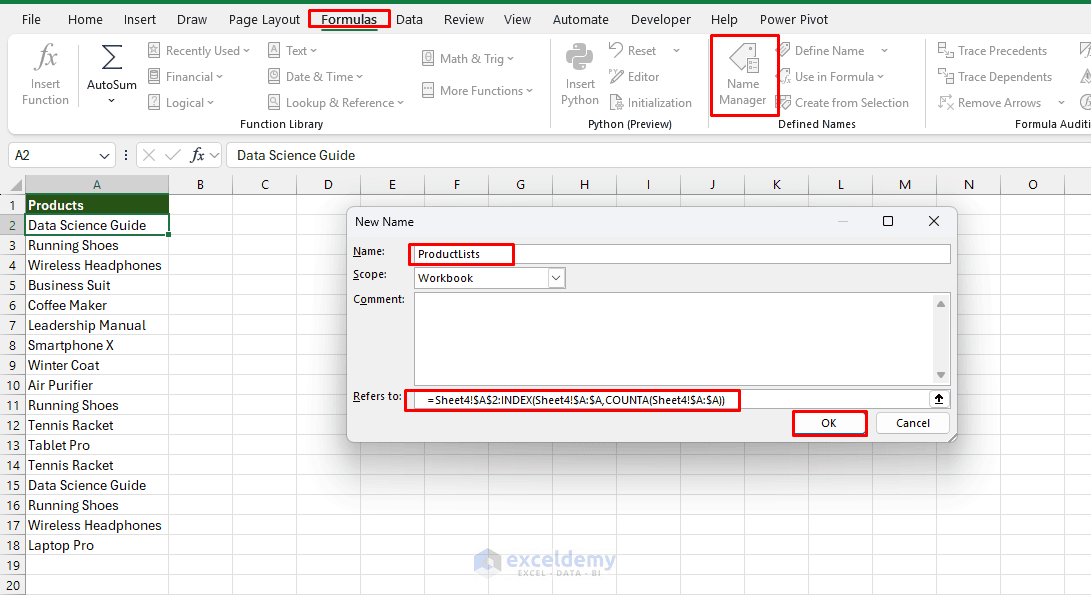
- Go to the Formulas tab >> select Name Manager >> select New
- Name it something like DynamicList
- In Refers to:, use the INDEX method (more stable than OFFSET, which is volatile and can slow down large workbooks):
=Sheet4!$A$2:INDEX(Sheet4!$A:$A,COUNTA(Sheet4!$A:$A))
This starts at A2 and extends down to the last non-blank cell in column A, recalculating every time COUNTA changes.
- Click OK
Step 2: Use the Named Range in Data Validation
- Select your drop-down cell
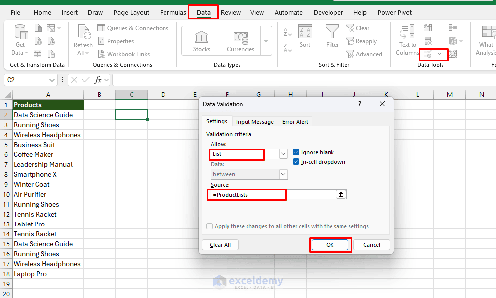
- Go to the Data tab >> select Data Validation >> select List
- In “Source,” type:
=DynamicList
- Click OK
Test:
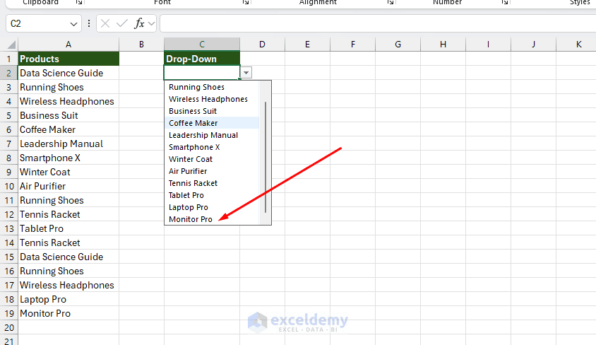
- Add a new item at the bottom of column A
- Click the drop-down — it’s there
Why INDEX instead of OFFSET: OFFSET is a volatile function — it recalculates on every single change to the workbook, even unrelated ones, which can slow things down in large files. INDEX is not volatile, so it only recalculates when its actual inputs change. Same result, better performance.
Which Method Should You Use?
| Situation | Best Method |
| You’re on Excel 2016–2019, no dynamic arrays | Method 1 (Table) |
| You’re on Excel 365 and want auto-sorted, deduplicated lists | Method 2 (UNIQUE/SORT) |
| You’re on an older Excel version with no tables allowed | Method 3 (INDEX named range) |
| You want the simplest possible setup | Method 1 (Table) — always start here |
Common Mistakes to Avoid
- Referencing the whole column: Referencing a full column directly in Data Validation instead of using a table or named range includes blank cells and shows empty items in the drop-down.
- Using OFFSET on large datasets: It’s volatile and can noticeably slow down larger workbooks.
- Forgetting to rename the table: If you have multiple tables, names like Table1 and Table2 get confusing fast. Rename each one to something meaningful right after creating it.
- Typing values directly into Data Validation without proper referencing: Data Validation lists using named ranges work across sheets, but manually typed lists do not.
Conclusion
You can follow any of these methods to build a dynamic drop-down list that updates itself. Once set up, you’ll never have to manually edit a drop-down’s source range again — just add data, and the list keeps itself current. If you want, you can even combine all three approaches to make things more user-friendly: use an automatically expanding Excel table to capture new records, FILTER to remove blanks, UNIQUE to remove duplicates, and SORT to keep the list organized. Referencing the spilled results through a named range then creates a drop-down that expands or contracts automatically as the source data changes.
Get FREE Advanced Excel Exercises with Solutions!