
An A/B test helps you compare two versions of a website, landing page, email, or marketing campaign to see which performs better. But comparing conversion rates alone isn’t enough. You also need to determine whether the difference is statistically significant or could simply be due to random variation.
In this tutorial, we’ll show you how to analyze an A/B test in Excel, from raw data to a one-page decision summary you can hand to a manager.
Step 1: Prepare the Raw A/B Test Data in Excel
Suppose an online store wants to test whether a redesigned checkout button increases purchases. Visitors are randomly assigned to one of two groups:
- Version A (Control): The original checkout button.
- Version B (Variant): The redesigned checkout button.
The primary goal is to increase the percentage of visitors who make a purchase. We’ll also examine revenue per visitor to check whether higher conversions translate into higher average revenue.
Our example dataset contains 4,000 visitors, with 2,000 in each group.
| Column | Header | Description |
|---|---|---|
| A | VisitorID | Unique ID for each visitor |
| B | Variant | A (Control) or B (Variant) |
| C | Converted | 1 if purchased, 0 otherwise |
| D | RevenuePerVisitor | Revenue generated by that visitor |
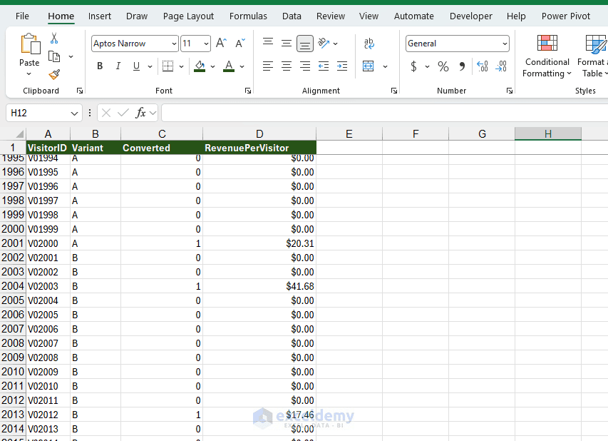
Before performing the analysis, check that each visitor appears only once, the Variant column contains valid group labels, and Converted contains only 0 or 1. For this example, every non-purchasing visitor has $0 revenue. Run three quick checks, because bad data breaks every number that follows:
- Duplicates: Select column A and use Data >> Remove Duplicates, or compare =COUNTA(A2:A4001) with the number of unique IDs. One visitor counted twice breaks the independence assumption.
- Valid Values: Confirm that the Converted column contains only 0 and 1. The formula =COUNTIFS(C2:C4001,”<>0″,C2:C4001,”<>1″) should return 0.
- Split Sanity: If you planned a 50/50 split and see 5,000 versus 4,100 visitors, something went wrong in the assignment. Investigate before trusting the result.
Step 2: Calculate Conversion Rates and Uplift
Create a new worksheet named Analysis.
- Enter Metric in cell A5
- Enter the variant labels A in cell B5 and B in cell C5
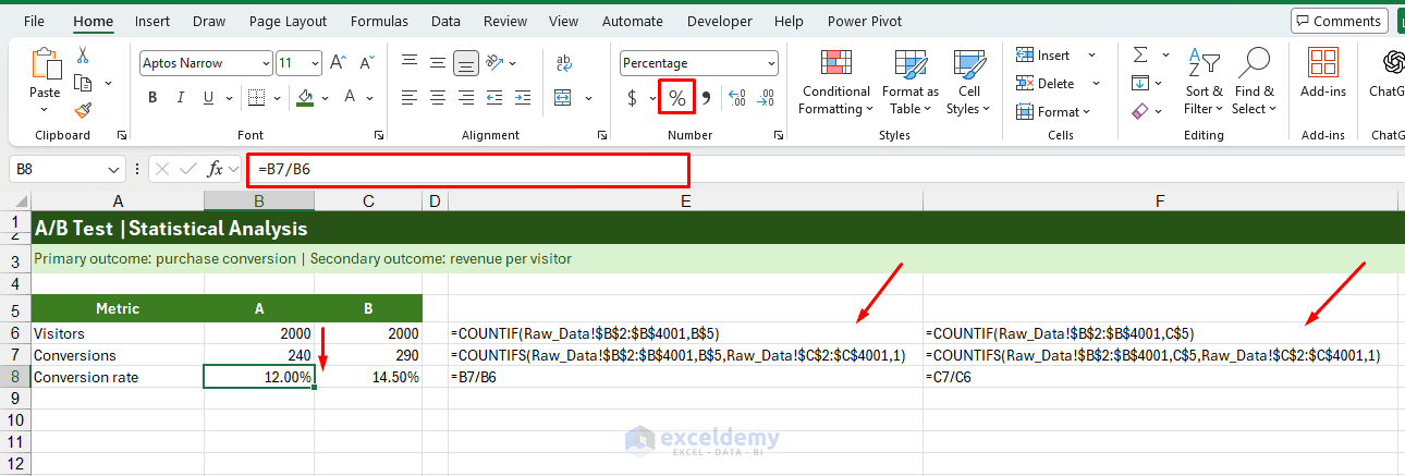
- Then add Visitors, Conversions, and Conversion Rate in cells A6:A8
Count Visitors and Conversions:
- In B6, count visitors:
- Copy the formula across to C6 to count Version B
=COUNTIF(Raw_Data!$B$2:$B$4001,B$5)This counts the number of visitors assigned to Version A.
- In B7, count conversions:
- Copy the formula to C7
=COUNTIFS(Raw_Data!$B$2:$B$4001,B$5,Raw_Data!$C$2:$C$4001,1)The formula counts only visitors who belong to the selected group and have a Converted value of 1.
- In B8, calculate the conversion rate:
=B7/B6- Copy across to C8 and format both cells as Percentage
Calculate Absolute and Relative Uplift
There are two ways to measure the difference between the groups. Absolute uplift measures the difference between their conversion rates.
- In F7, enter the following formula and format it as a Percentage:
=C8-B8Relative uplift measures the percentage improvement compared with the original rate.
- In F8, insert the following formula and format it as a Percentage:
=C8/B8-1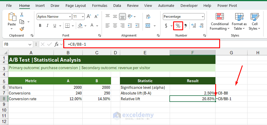
Version B therefore has a conversion rate that is 2.5 percentage points higher, representing a 20.83% relative improvement over Version A.
The difference is promising, but a higher observed conversion rate doesn’t automatically mean the new design is better. We need to assess the uncertainty around the results.
Step 3: Calculate 95% Confidence Intervals
A confidence interval provides a range of plausible values for the underlying conversion rate or the difference between two rates, based on sampling uncertainty. We’ll calculate 95% confidence intervals for each group and then for the difference between them.
Calculate Confidence Intervals for Individual Groups
- First, enter 0.05 in cell F6 as the significance level (alpha)
- This corresponds to a 95% confidence level
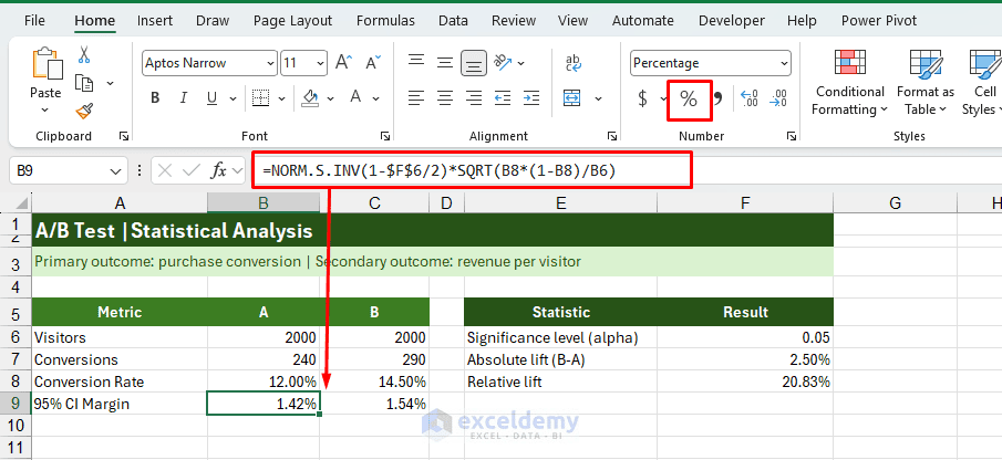
- In B9, calculate the margin of error:
=NORM.S.INV(1-$F$6/2)*SQRT(B8*(1-B8)/B6)Here, NORM.S.INV provides the critical z-value, and the SQRT term calculates the standard error.
- In B10, calculate the lower limit:
=B8-B9- In B11, calculate the upper limit:
=B8+B9- Copy B9:B11 across to C9:C11 and format all six cells as Percentage
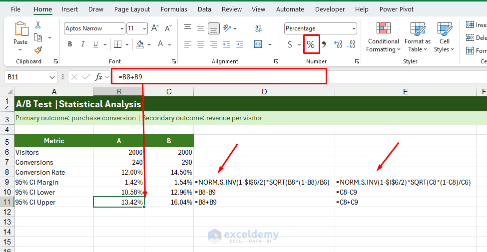
These are large-sample normal-approximation intervals, suitable as an introductory approach for this example. For small samples or conversion rates near 0% or 100%, Wilson intervals are generally more reliable.
Calculate the Confidence Interval for the Difference
For an A/B decision, the confidence interval of the difference between B and A is especially useful.
- In F9, calculate the unpooled standard error:
=SQRT(B8*(1-B8)/B6+C8*(1-C8)/C6)- In F10, calculate the lower limit:
=F7-NORM.S.INV(1-F6/2)*F9- In F11, calculate the upper limit:
=F7+NORM.S.INV(1-F6/2)*F9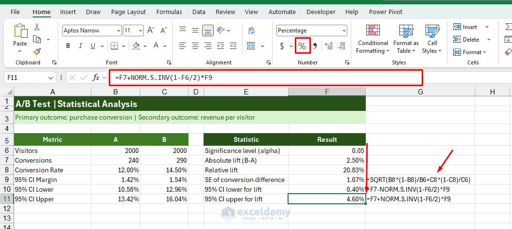
The 95% confidence interval for the difference is approximately +0.40 to +4.60 percentage points.
Observed conversion uplift and its 95% confidence interval: The interval is entirely above zero, providing evidence of a positive difference at the 5% significance level. The interval suggests that the true conversion improvement could be much smaller or larger than the observed 2.5 percentage points. It does not mean that there is a 95% probability the fixed true effect lies inside this particular calculated interval.
Step 4: Run a Two-Proportion Z-Test in Excel
A two-proportion z-test determines whether the conversion rates of two independent groups differ significantly. Since the outcome is binary (converted or did not convert), this is the appropriate basic test for our primary metric.
We test:
- Null hypothesis (H₀): The conversion rates of A and B are equal
- Alternative hypothesis (H₁): Their conversion rates differ
We’ll use a two-sided test at the 5% significance level. Excel doesn’t have a dedicated two-proportion z-test worksheet function, so we’ll calculate the statistic using built-in functions.
Calculate the Pooled Conversion Rate
- In F12, enter:
=(B7+C7)/(B6+C6)This combines the conversions from both groups and divides by the total number of visitors.
Calculate the Pooled Standard Error
- In F13, enter:
=SQRT(F12*(1-F12)*(1/B6+1/C6))We use the pooled standard error for the hypothesis test because the null hypothesis assumes equal underlying conversion rates. This differs from the unpooled standard error used for the confidence interval.
Calculate the Z-Statistic
- In F14, enter:
=F7/F13Calculate the Two-Sided P-Value
- In F15, enter:
=2*(1-NORM.S.DIST(ABS(F14),TRUE))NORM.S.DIST returns the cumulative standard normal probability when its second argument is TRUE. We multiply the upper-tail probability by two because the test is two-sided.
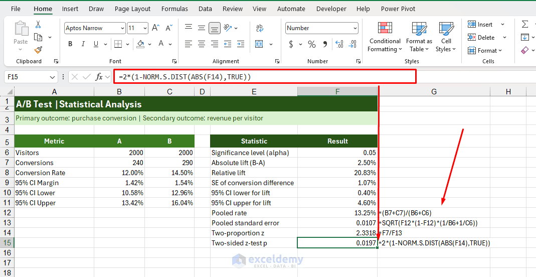
- Z-statistic: 2.3318
- Two-sided p-value: 0.0197
Interpretation: Since 0.0197 is less than our significance level of 0.05, we reject the null hypothesis of equal conversion rates. The experiment provides statistically significant evidence that the two versions perform differently, with Version B showing a higher conversion rate.
A p-value of 0.0197 does not mean there is a 1.97% probability that the null hypothesis is true. Rather, it measures how unusual a result at least this extreme would be if the two underlying conversion rates were equal.
Step 5: Run a T-Test to Compare Revenue per Visitor
Conversion rate tells us how many visitors purchased, but it doesn’t tell us how much revenue each version generates. Version B might increase the number of orders while reducing the average order value. We’ll therefore compare revenue per visitor as a secondary metric.
Calculate Average Revenue Per Visitor:
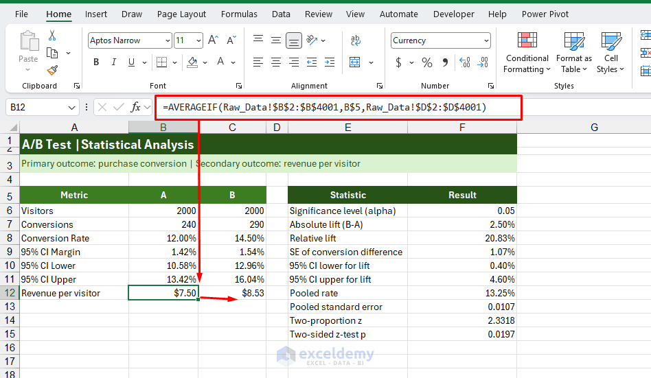
- In B12, enter the following formula and copy it across to C12:
=AVERAGEIF(Raw_Data!$B$2:$B$4001,B$5,Raw_Data!$D$2:$D$4001)The results are approximately $7.50 for Control and $8.53 for Variant. Importantly, revenue per visitor includes the zero-revenue visitors. Excluding them would instead calculate the average order value among purchasing visitors.
Perform a Two-Sample T-Test:
Since the revenue values are numeric, we can use T.TEST to compare the group means.
- In F16, enter:
=T.TEST(Raw_Data!$D$2:$D$2001,Raw_Data!$D$2002:$D$4001,2,3)The last two arguments determine the test:
- 2 specifies a two-tailed test
- 3 specifies a two-sample unequal-variance test, also known as Welch’s t-test
This formula works because our practice data is sorted into two contiguous groups. If your actual data has the groups mixed together, you can use this alternative in Excel 2021 or later, including Excel for Microsoft 365:
=T.TEST(
FILTER(Raw_Data!D2:D4001,Raw_Data!B2:B4001="A"),
FILTER(Raw_Data!D2:D4001,Raw_Data!B2:B4001="B"),
2,3)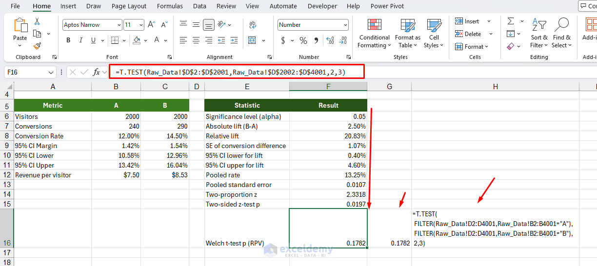
Since 0.1782 is greater than 0.05, the revenue difference is not statistically significant. This doesn’t prove the revenues are equal; the test simply doesn’t establish a difference.
Revenue data is often skewed, with many zero values and a few large purchases. Welch’s t-test is a useful introductory comparison, but for heavily skewed revenue metrics, a visitor-level bootstrap confidence interval can provide an additional robustness check.
Step 6: Create a One-Page A/B Test Decision Summary
Our calculations are complete. The final step is to present the findings in a form that a manager or stakeholder can understand without examining every formula.
- Create a new worksheet named Decision_Summary
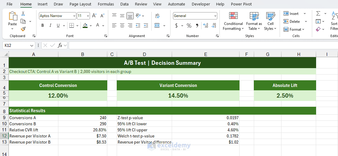
- Arrange the main metrics, statistical results, and recommendation as follows:
A/B Test Decision Summary
Make the Decision Summary Dynamic
Rather than entering the results manually, link each metric to the Analysis worksheet.
For example, to display the conversion rate for Version B:
=Analysis!C8To return a short statistical decision:
=IF(AND(Analysis!F15<Analysis!F6,Analysis!F14>0),"Significant conversion uplift","Insufficient evidence of uplift")To automatically generate a recommendation:
=IF(AND(Analysis!F15<Analysis!F6,Analysis!F14>0),"Consider staged rollout after guardrail checks","Hold variant and review results")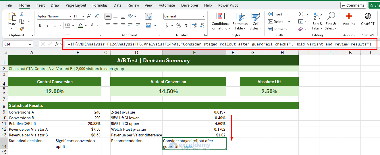
Recommendation: Consider a staged rollout of Version B, provided the experiment passes data-quality checks and no predefined business guardrails are violated. Monitor revenue per visitor during the rollout.
Statistical evidence supports improved conversions but does not yet establish improved revenue. These formulas provide a starting point, but the final business decision should also consider revenue, costs, technical performance, and experiment validity.
Step 7: Check the Results Before Making a Decision
A statistically significant result is useful only when the experiment itself is reliable. Before approving a rollout, review the following checks:
- Data Quality: Confirm unique visitor IDs, accurate conversion events, complete revenue records, and consistent attribution.
- Randomization: Check that traffic was assigned according to the planned allocation. An unexpected sample-ratio mismatch can indicate an implementation or logging problem.
- Test Design: Check that the planned sample size and test duration were met, that primary metrics were defined in advance, and that repeated significance checks haven’t inflated the false-positive risk.
- Business Impact: Evaluate the magnitude of the uplift, costs, revenue guardrails, and whether the result is economically meaningful.
In this example, the conversion improvement is statistically significant, but the revenue finding is inconclusive. That is why the recommendation is a cautious, monitored rollout rather than an unconditional release.
Conclusion
By following this tutorial, you can analyze an A/B test in Excel from raw data to a decision. Analyzing an A/B test in Excel involves more than finding the version with the highest conversion rate. A complete analysis should quantify the improvement, estimate its uncertainty, test the relevant hypotheses, and translate the statistical evidence into a business decision. Excel makes it possible to analyze an A/B test using built-in formulas. By calculating conversion rates, confidence intervals, and p-values, you can determine whether an observed difference is supported by statistical evidence.
In our example, Version B increases conversions significantly, but the revenue results remain inconclusive. A one-page decision summary helps communicate both findings and supports a more informed rollout decision.