
When you work with several related datasets in Excel, putting everything into one large table is not always the best approach. Customer information may belong in one table, product information in another, and individual transactions in a third. Excel Table Relationships let you connect multiple tables the way a database does, through shared key columns, so you can analyze fields from multiple tables in the same PivotTable without repeatedly bringing data into one table with VLOOKUP or XLOOKUP.
In this tutorial, we will cover all about Excel table relationships. Excel relationships are particularly useful for large datasets, PivotTables, reporting models, and workbook structures that resemble relational databases.
What Are Table Relationships?
A relationship is a link between two tables based on a column they have in common. Instead of copying data from one table into another, Excel remembers that “this column in Table A corresponds to that column in Table B” and uses that connection on the fly whenever you build a report. One side is typically a primary key (unique values) and the other a foreign key (values that can repeat).
Every relationship has two sides:
- Lookup Table (also called the “one” side or dimension table): Contains a column of unique values, no duplicates. This is your reference list, like a Customers table where each Customer ID appears exactly once.
- Data Table (also called the “many” side or fact table): Contains a column with repeating values that point back to the lookup table. This is your transactional data, like an Orders table where the same Customer ID appears once per order.
- Column names do not have to match, but the data types must be compatible.
Relationships live inside the workbook’s Data Model. They do not alter the original tables on the worksheets.
Prerequisite – Get Your Data Ready
Before creating a relationship, each dataset needs to be an actual Excel Table (not just a range).
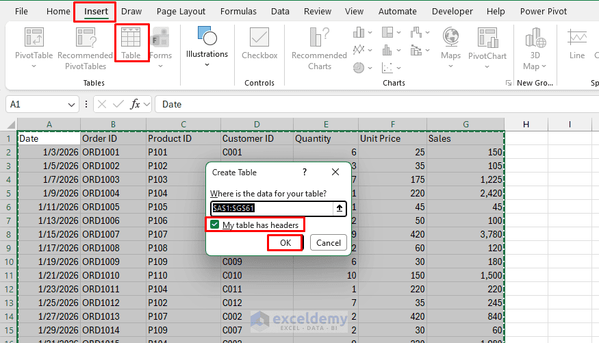
- Click any cell in your dataset
- Go to the Insert tab >> select Table or press Ctrl + T
- Confirm “My table has headers” >> click OK
- Go to the Table Design tab >> give it a clean, descriptive name (e.g., Sales, Products, Customers)
- Avoid spaces and generic names like Table1, since you will be referencing these names constantly
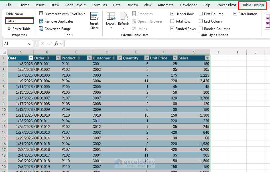
Repeat for every table you want in the model. This step matters: Excel’s Data Model can only build relationships between proper Tables (or Power Query queries), not plain cell ranges.
Method 1: Manual Creation via the Relationships Dialog
This is the more reliable method, especially when column names differ or you have several tables to connect at once.
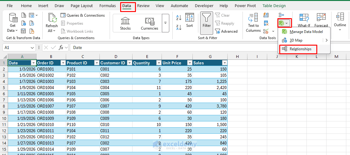
- Go to the Data tab >> from the Data Tools group >> click Data Model >> select Relationships
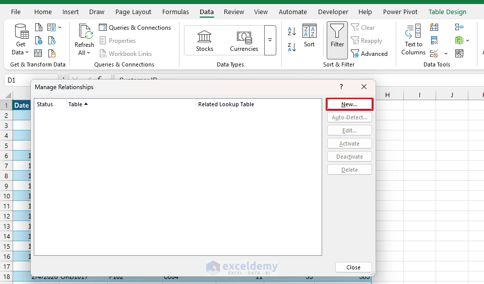
- In the Manage Relationships window, click New
- Fill in the four fields:
- Table: The table on the “many” side (e.g., Sales)
- Column (Foreign): The shared key in that table (e.g., Product ID; this column can have duplicates)
- Related Table: The lookup table on the “one” side (e.g., Products)
- Related Column (Primary): The shared key in the lookup table (e.g., Product ID; this column must be unique, with no duplicates and no blanks)
- Click OK
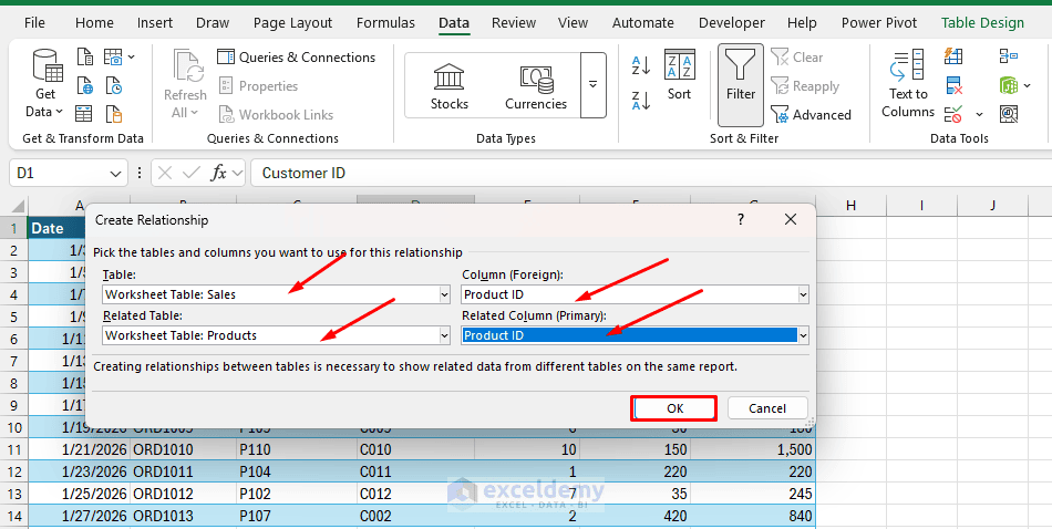
- Repeat New for any additional relationships (e.g., linking Sales to a Customers table via Customer ID)
- Click Close
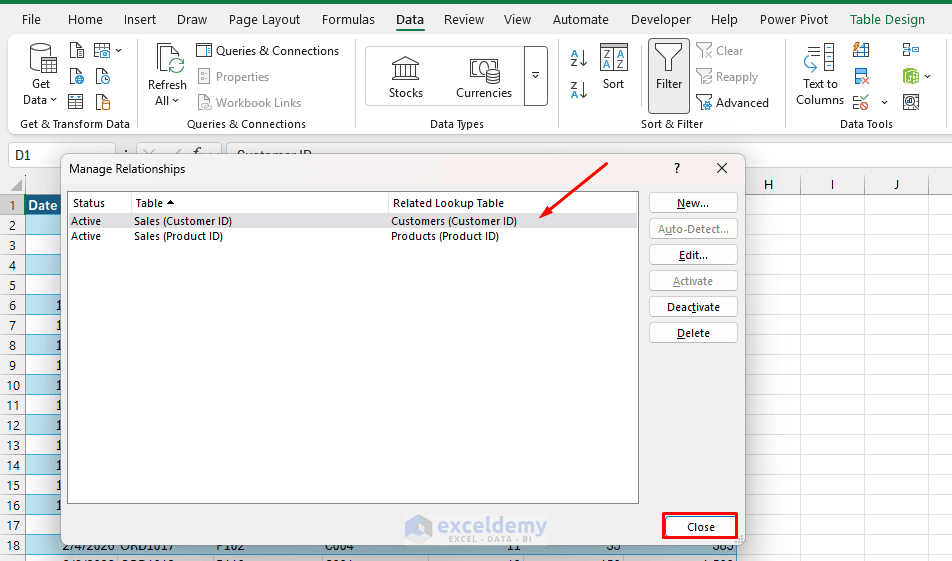
Excel is strict about direction here: the “Related Column” must contain unique values. If Excel throws an error when creating the relationship, it is almost always because the column you chose as the primary/related side actually contains duplicates.
Method 2: Auto-Detect via PivotTable
The fastest way to create a relationship is to let Excel find it for you while building a PivotTable.
- Click inside one of your Tables
- Go to the Insert tab >> select PivotTable
- Choose your location: New Worksheet
- Check Add this data to the Data Model
- Click OK to place the PivotTable
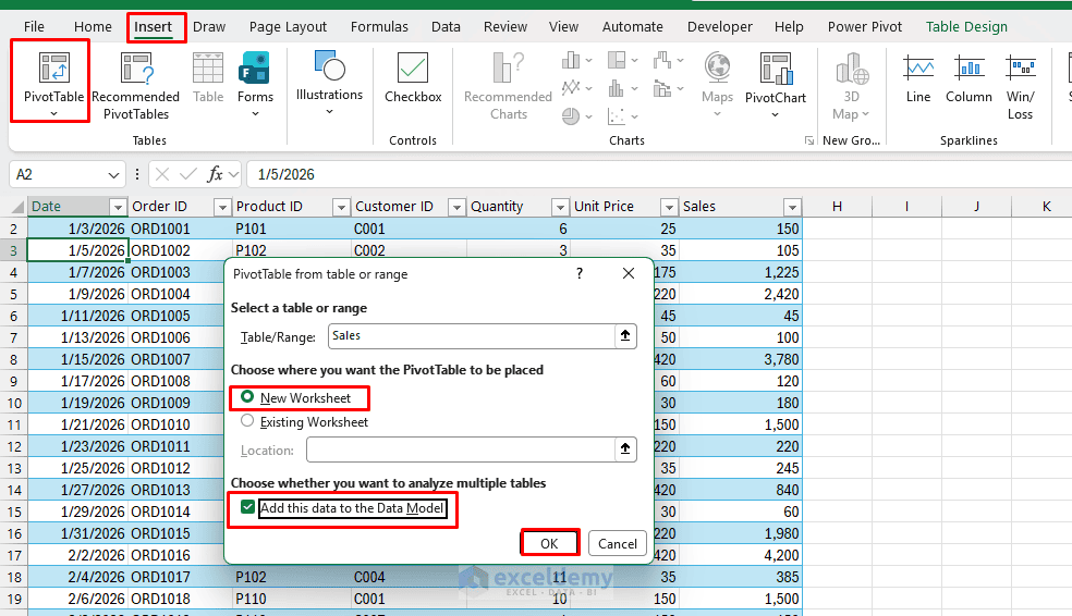
- In the PivotTable Fields pane, click All at the top instead of Active; this reveals every table in your workbook, not just the one you started from
- Drag a field from Sales and a field from Customers into the same PivotTable (e.g., Sales Total from Orders, Product Name from Products)
- A yellow banner appears: “Relationships between tables may be needed.”
- Click Auto-Detect
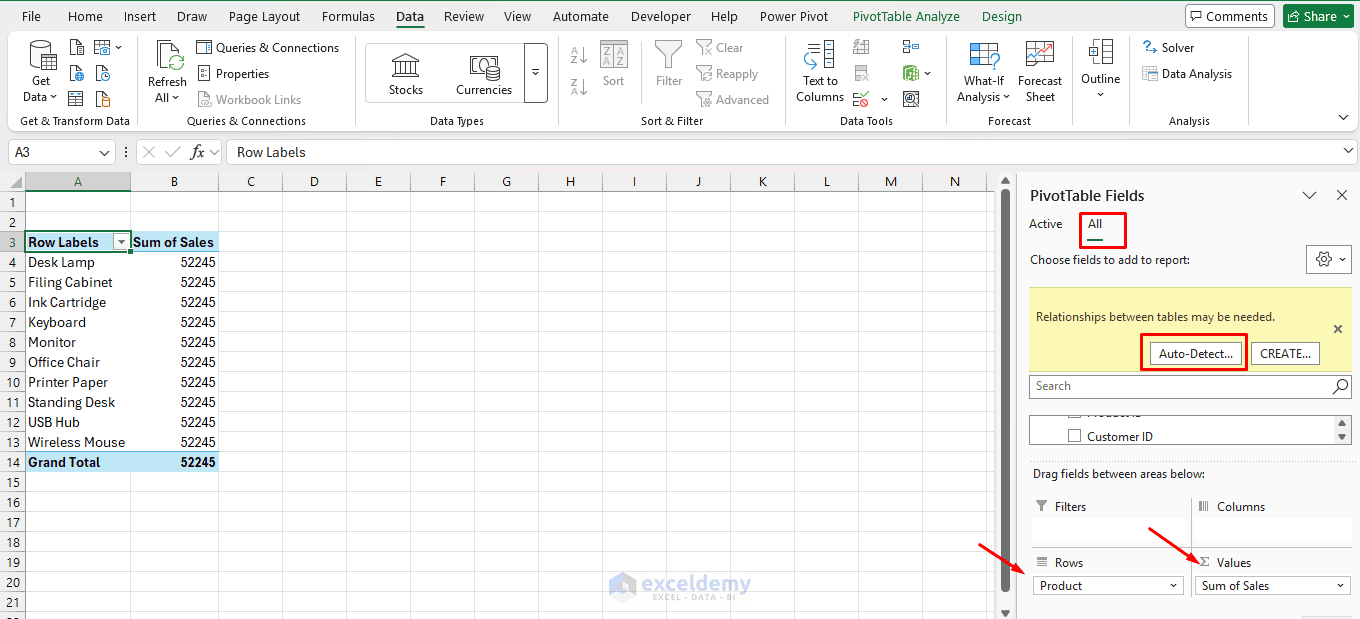
- Excel scans for columns with matching names and compatible data (like Product ID in both tables) and creates the relationship automatically
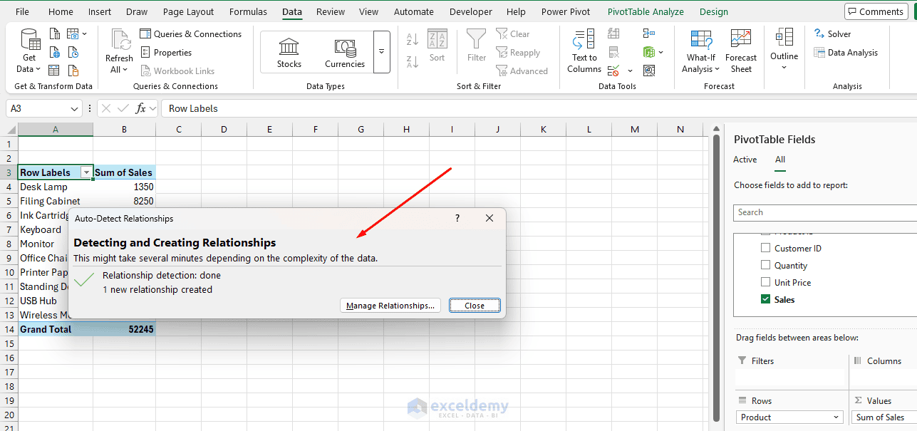
If Auto-Detect does not find a match — usually because the key columns have different names — click Create in that same banner instead, and you will land in the manual dialog covered next.
Method 3: Diagram View (Power Pivot)
If you have the Power Pivot add-in enabled, you will get a visual canvas for managing relationships. It is more convenient.
- Go to the Power Pivot tab >> select Manage
- It will open the Power Pivot window
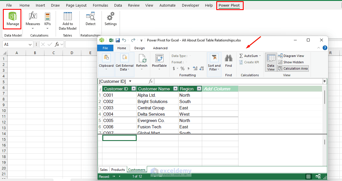
- Go to the Home tab >> select Diagram View
- Each table appears as a box listing its columns
- Click and drag from the key column in one table directly onto the matching key column in another table
- A connecting line appears, representing the relationship
- Double-click the line at any time to edit or verify it
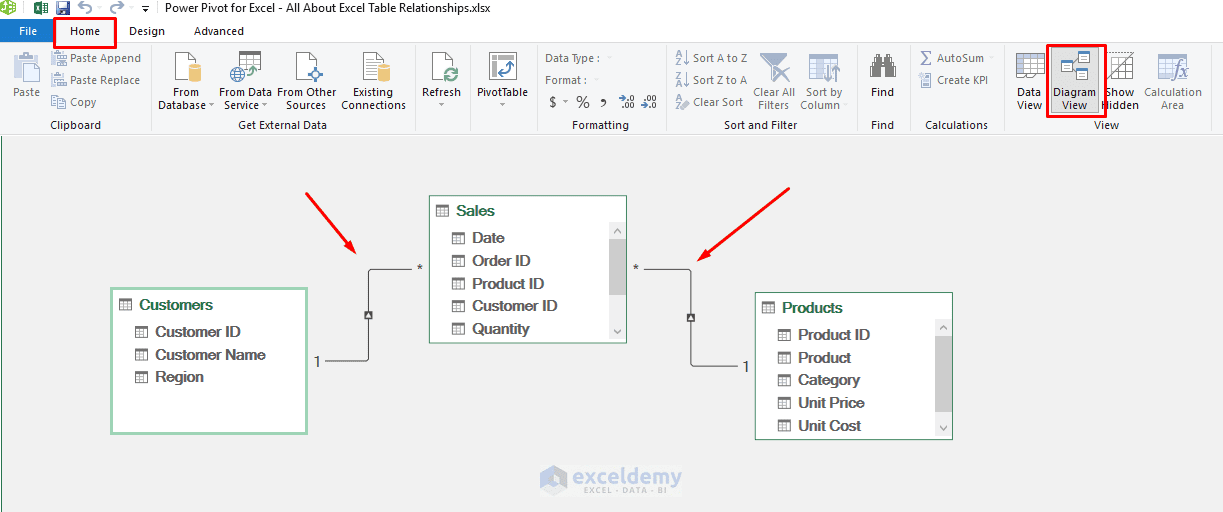
Diagram View is the best option once you are working with more than three or four tables, since it lets you see the entire model’s structure at a glance instead of reading through a list.
Tip: If not available, go to File → Options → Add-ins → COM Add-ins → check Microsoft Power Pivot for Excel
Working With Relationships After Creation
Building PivotTables and PivotCharts Across Tables
The main reason for creating Excel relationships is to analyze fields from several tables together. After creating the relationships, insert a PivotTable based on the workbook’s Data Model.
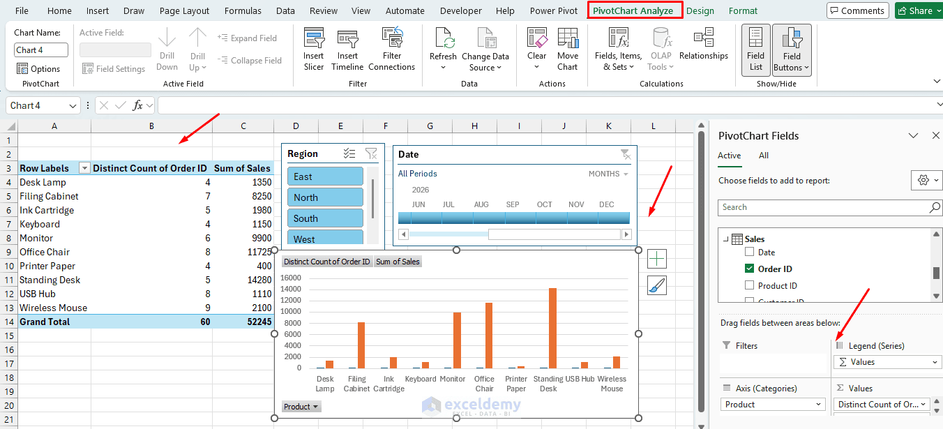
- Create a PivotTable based on the Data Model
- The Fields list shows every table in the All section
- Drag any field from any related table into Rows, Columns, Values, or Filters
- Slicers and Timelines work across the relationships
- You gain Distinct Count as a summarization option (unavailable in ordinary PivotTables)
- Insert PivotChart
Adding Calculated Fields with DAX
In Power Pivot’s Manage window, you can write DAX measures that travel across relationships (e.g., using RELATED or RELATEDTABLE).
- Go to the Power Pivot tab >> click Manage
- You can create DAX measures that calculate values from related tables
Total Sales:=SUMX( Sales, Sales[Quantity] * Sales[Unit Price] )
Total Cost:=SUMX(Sales,RELATED(Products[Unit Cost]) * Sales[Quantity])
Total Profit:=[Total Sales] - [Total Cost]
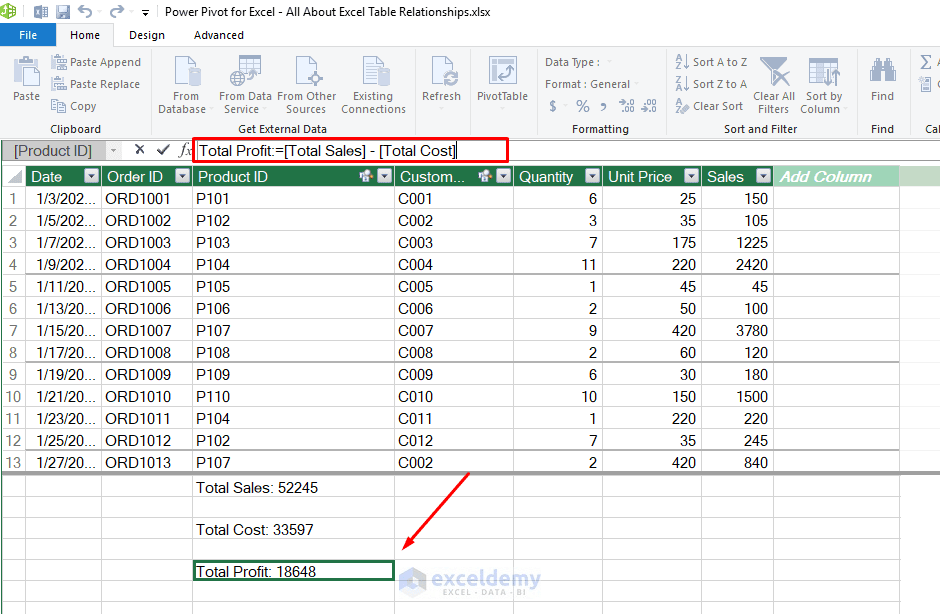
The RELATED function follows the relationship between Sales[Product ID] and Products[Product ID] to retrieve the corresponding unit cost for each sales transaction.
These calculations demonstrate how DAX can use relationships between tables without copying product information into the Sales table.
Using Cube Functions
Functions such as CUBEVALUE and CUBEMEMBER can retrieve values directly from the Excel Data Model and display them in regular worksheet cells. This is useful for creating custom dashboards without relying on the standard PivotTable layout.
- Suppose you want to get the Electronics member from the Category field. Use the following formula:
=CUBEMEMBER("ThisWorkbookDataModel","[Products].[Category].[Electronics]")
- Next, use CUBEVALUE to return a measure for that member:
=CUBEVALUE("ThisWorkbookDataModel","[Measures].[Total Sales]",B2)
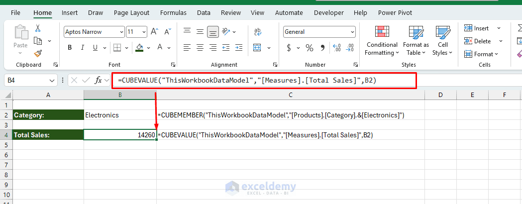
This approach gives you more control over where Data Model results appear in a worksheet.
Editing or Removing a Relationship
- Go to the Data tab >> click Data Model >> select Relationships
- Click Edit or Delete
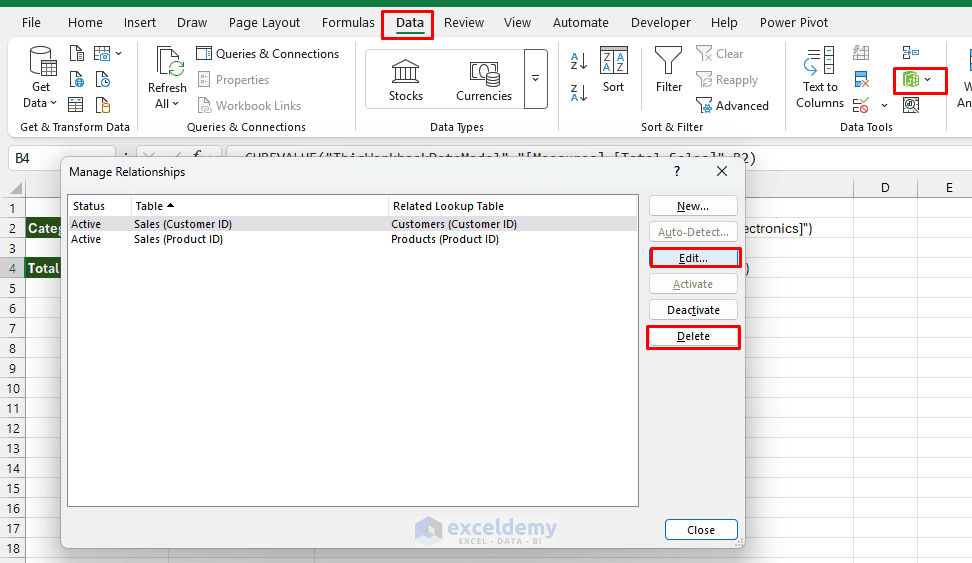
Deleting a relationship does not delete any data; it only breaks the connection, so any PivotTable relying on it will show blank or mismatched values until you rebuild the link.
Refreshing Data
If your source tables come from Power Query or external connections,
- Go to the Data tab >> select Refresh All
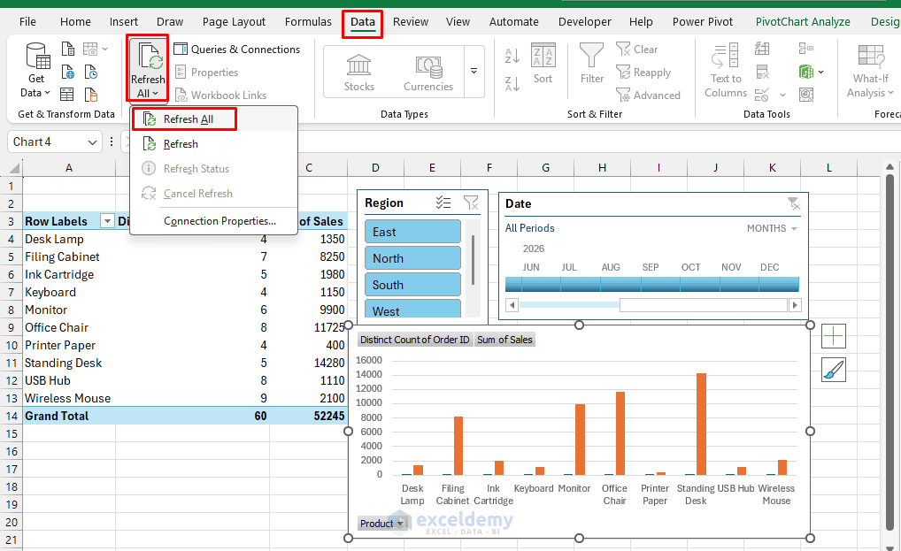
Relationships persist through a refresh as long as the key columns and table names do not change.
Types of Relationships
One-to-Many: This is the most common relationship type supported in the Excel Data Model. One value in a lookup table can match many rows in another table. For example, one customer can place many orders, or one product can appear in many sales records.
One-to-One: Each value in one table matches only one value in another table. For example, one employee may have one matching row in an Employee Details table.
Many-to-Many: Both tables can contain repeated values. For example, one student can take many courses, and one course can have many students. The Data Model does not natively support many-to-many relationships through the simple UI — you would need bridge tables or more advanced modeling.
Why Use Relationships Instead of VLOOKUP/XLOOKUP?
| Particulars | Lookup Functions | Data Model Relationships |
| Setup | Formula in every row | One-time relationship definition |
| File size | Grows with duplicated lookup columns | No duplication; data stays in its own table |
| Performance on large data | Slows down significantly (millions of formulas) | Built for large datasets (VertiPaq engine) |
| Maintenance | Formulas break if columns move | Relationship persists independent of layout |
| Multi-table analysis | Requires nested/chained lookups | Native; pull fields from any related table into one PivotTable |
| Best for | Small, simple, one-off lookups | Recurring reporting, dashboards, large datasets |
If you are building something you will refresh and reuse, like a monthly sales report, a dashboard, or an inventory tracker, relationships almost always win.
Common Problems with Excel Table Relationships
- Relationship Cannot Be Created: Trying to relate two columns that both contain duplicates. Check the lookup column for duplicate values.
- Relationships Option Is Unavailable: Make sure your workbook contains at least two suitable tables. Microsoft notes that the Relationships command may not be available when the workbook contains only one table.
- PivotTable Shows “Relationships Between Tables May Be Needed”: This means you are attempting to use fields from tables that Excel cannot currently connect. Excel can detect that a relationship may be required, but it may not always know which columns should be used to create it.
- PivotTable Results Look Incorrect: Check whether you selected the correct key columns. Also check that IDs in the transaction table correspond to valid IDs in the lookup table.
Conclusion
By following this tutorial, you can learn all about Excel table relationships. Excel Table Relationships allow you to connect multiple tables through common fields without combining everything into one oversized worksheet. The most important concept is the one-to-many relationship. Keep unique information such as Customers and Products in separate lookup tables, keep transactions in a Sales or Orders table, and connect them using identifiers such as Customer ID and Product ID. For smaller worksheets, XLOOKUP or VLOOKUP may still be more convenient. But when you need to analyze several related tables in PivotTables, Excel’s Data Model and Table Relationships provide a much cleaner and more scalable structure.
Get FREE Advanced Excel Exercises with Solutions!