
A project timeline helps you see when tasks begin, how long they continue, which activities overlap, and when important milestones occur. Project timelines are one of those things people assume need specialized software or an add-in. Although dedicated project management software can create timelines automatically, Excel already includes several tools for building effective project schedules. You can create a project timeline in Excel using formulas, conditional formatting, charts, or SmartArt, without installing an add-in.
In this tutorial, we will show five different ways to build a project timeline in Excel without an add-in. Each suits a different situation, from formal client-facing decks to quick internal planning sheets.
Method 1: Create a Formula-Based Timeline Grid
A formula-based timeline places project dates across the worksheet and displays a symbol whenever a task is active on a particular date. This method is suitable for small projects when you want a simple daily schedule without creating a chart.
Step 1: Create the Date Headers
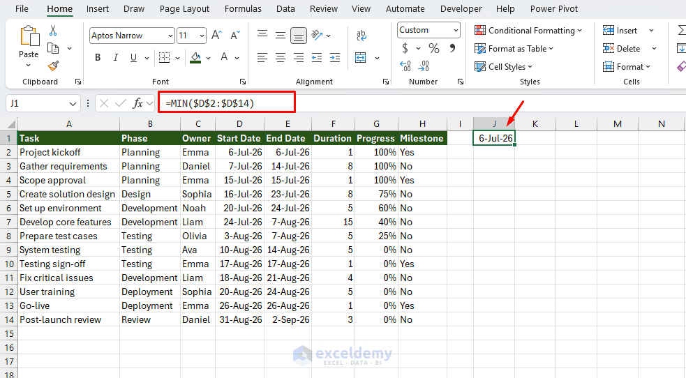
- Select cell J1 and enter the following formula:
=MIN($D$2:$D$14)
This returns the earliest project start date.
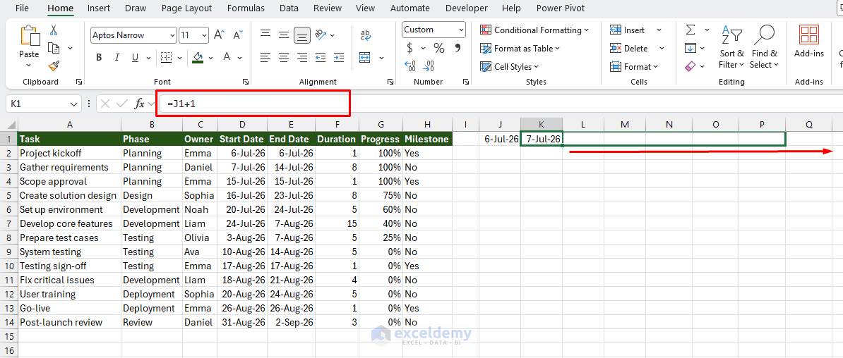
- Select cell K1 and insert the following formula:
=J1+1
- Drag the formula to the right until the timeline reaches the final project date.
- For this dataset, you can drag the formula through 2-Sep-26.
Format the date headers using a short date format such as:
d-mmm
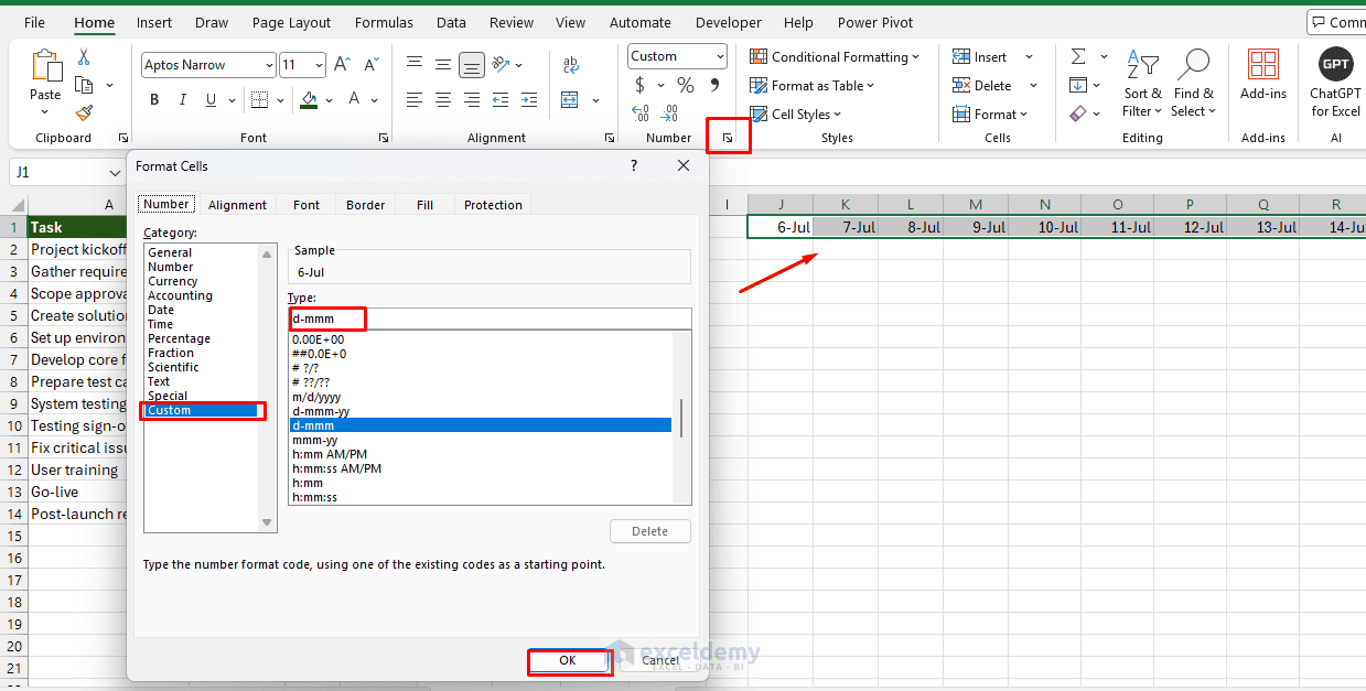
You can reduce the widths of the date columns so that the complete timeline fits on the screen.
Step 2: Display the Timeline Bars
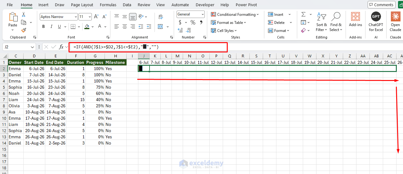
- Select cell J2 and enter the following formula.
- Drag the formula across the complete timeline and then down through row 14.
=IF(AND(J$1>=$D2,J$1<=$E2),"█","")
The formula checks whether the date in row 1 falls between the task's start and end dates. If both conditions are true, Excel displays a square symbol. Otherwise, Excel returns a blank cell.
Step 3: Format the Timeline
Select the timeline grid and apply the following formatting:
- Center the cell contents.
- Increase the font size slightly.
- Choose a font color for the timeline symbols.
- Reduce the widths of the date columns.
- Apply borders if you want to separate the days.
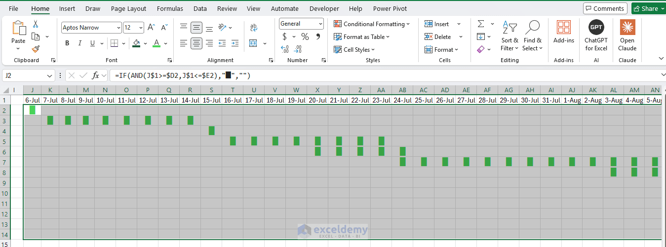
You can use a different symbol if required. For example:
=IF(AND(J$1>=$D2,J$1<=$E2),"●","")
This method creates a simple timeline that updates automatically when you change a task's start or end date.
Method 2: Build a Dynamic Timeline with Conditional Formatting
Conditional formatting creates colored timeline bars without placing symbols or values inside the cells. This method turns a grid of dates into a visual timeline by shading cells that fall within a task's date range, which is useful when you want a spreadsheet-native view that still looks visual without inserting any chart object at all.
You can also use separate colors to distinguish completed and remaining portions of each task.
Step 1: Create the Timeline Headers
Create the date headers in row 1 as shown in Method 1.
- In cell J1, enter the following formula:
=MIN($D$2:$D$14)
- In cell K1, enter the following formula.
- Drag the formula across the required date range until the last date.
=J1+1
Step 2: Highlight the Entire Planned Duration
- Select the timeline range J2:BP14.
- Go to the Home tab >> select Conditional Formatting >> select New Rule.
- Select Use a formula to determine which cells to format.
- Enter the following formula:
=AND(J$1>=$D2,J$1<=$E2)
- Click Format, select a light fill color, and click OK.
- Click OK.
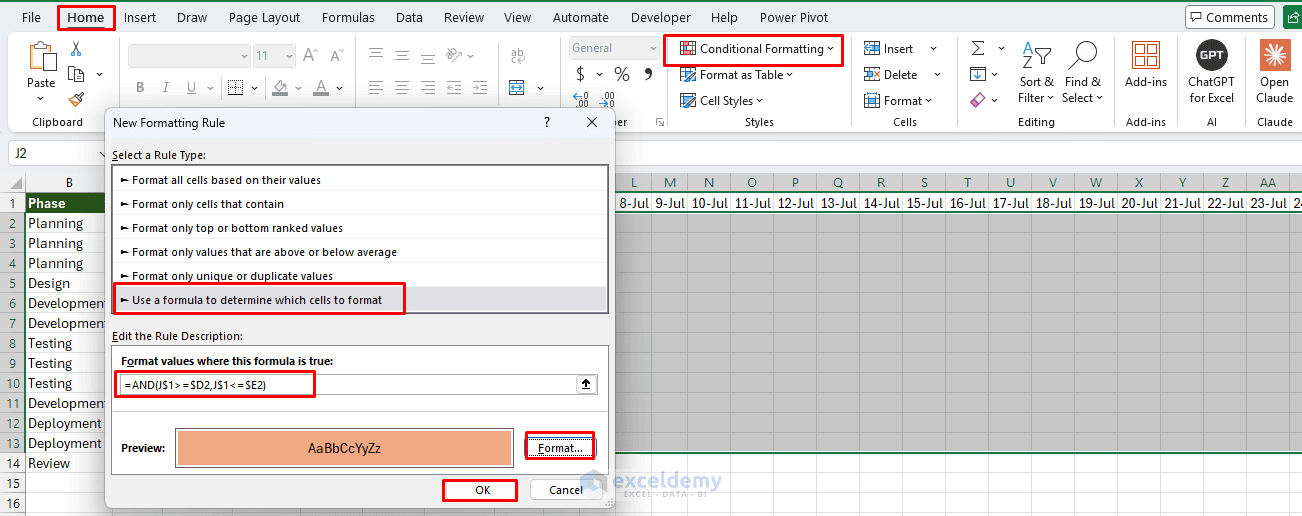
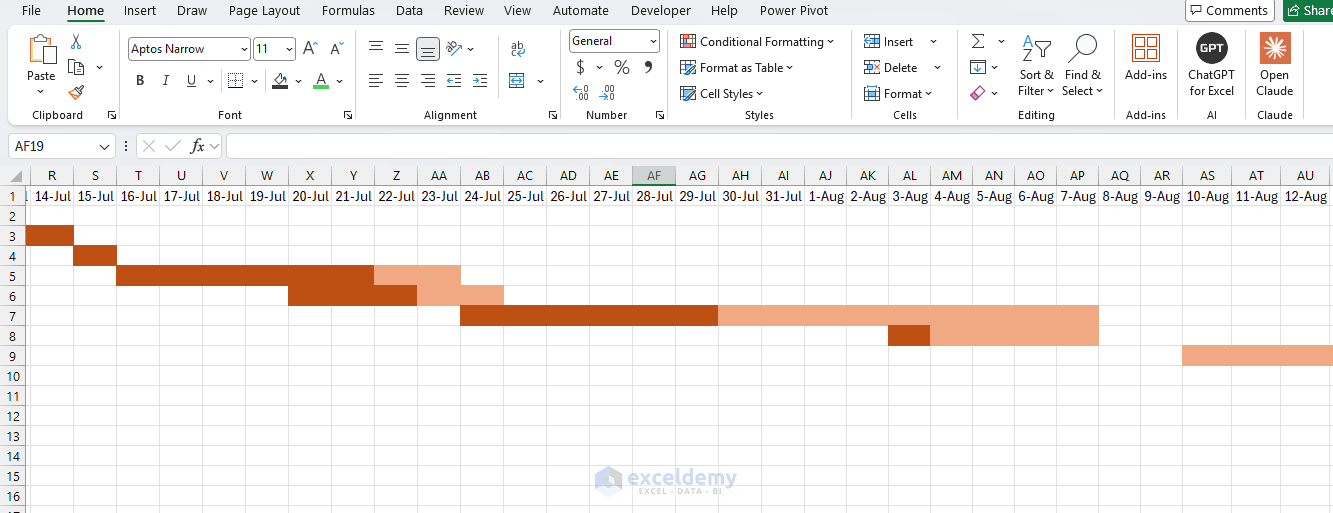
Excel will highlight every date between the task's start and end dates.
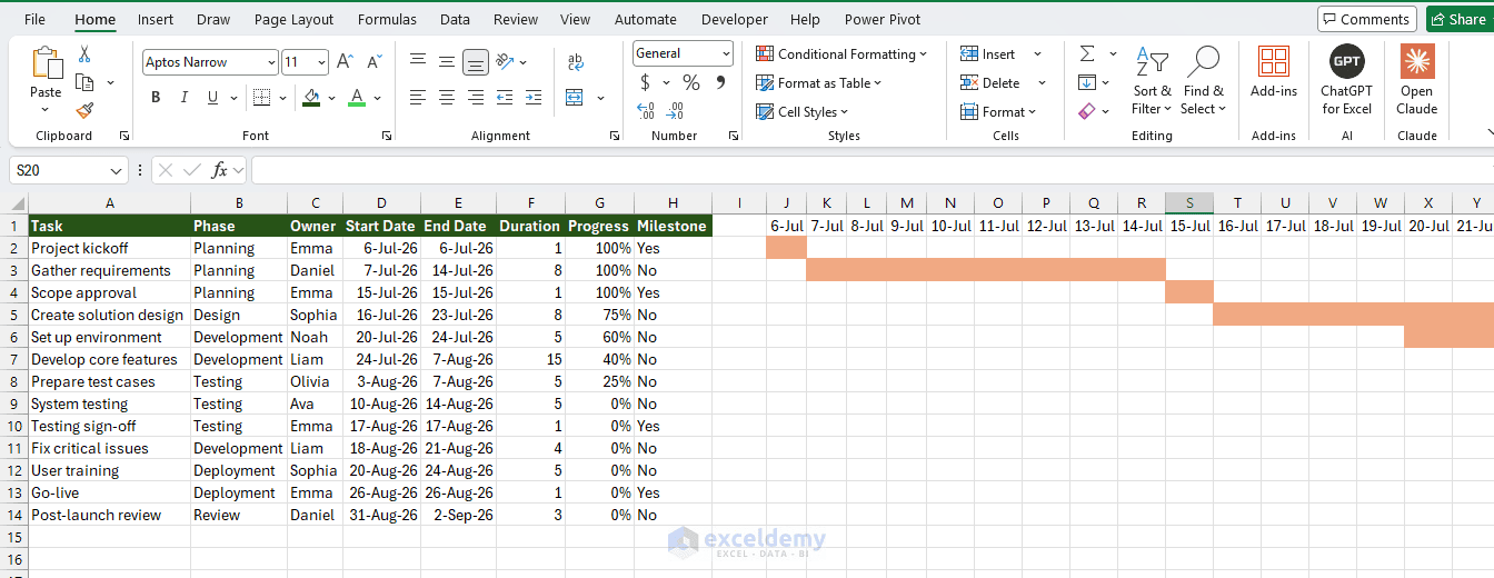
Step 3: Highlight the Completed Portion
With the same timeline range selected, create another conditional formatting rule.
Use this formula:
=AND(J$1>=$D2,J$1<=$D2+ROUND(($E2-$D2+1)*$G2,0)-1)
- Select a stronger fill color for completed work.
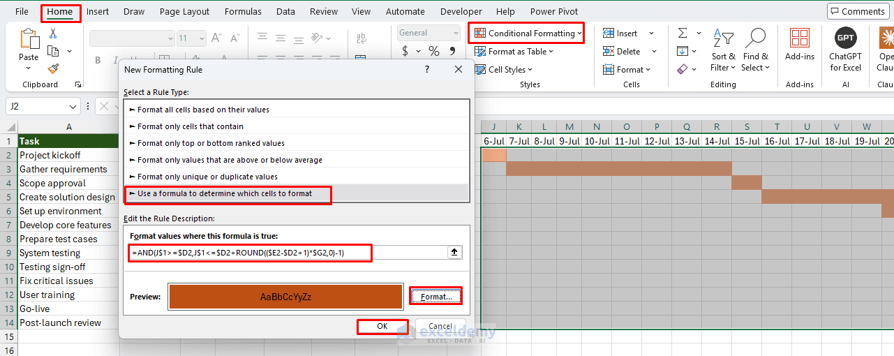
The formula calculates the number of completed days by multiplying the task duration by its progress percentage.
For example, if a task lasts eight days and is 75% complete, the first six days of the timeline bar will receive the completed-work color.
Optional: Highlight Today
Create another conditional formatting rule with:
=J$1=TODAY()
- Apply a border or a contrasting fill color.
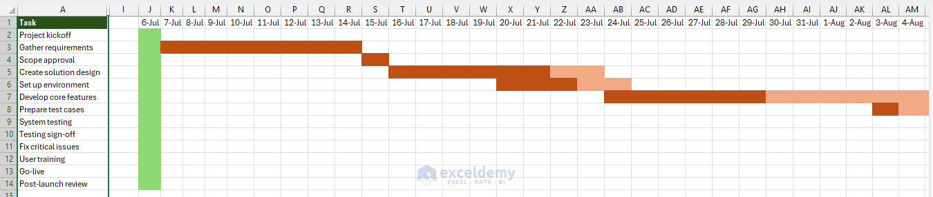
The timeline will then identify the current date automatically whenever the workbook is opened.
This conditional formatting method is among the most flexible options because the timeline updates immediately when dates or progress percentages change.
Method 3: Create a Gantt Chart with a Stacked Bar Chart
A Gantt chart displays tasks vertically and project dates horizontally. It is useful for reports, dashboards, and management presentations. Excel does not have a dedicated Gantt chart type, but you can create one using a stacked bar chart.
Step 1: Create the Helper Table
Create a helper table in an unused section of the worksheet with the following columns.
- Task:
=A2
- Start Date:
=D2
- Completed Days:
=ROUND(($E2-$D2+1)*$G2,0)
- Remaining Days:
=($E2-$D2+1)-L18
- Drag the formulas down until all project tasks appear in the helper table.
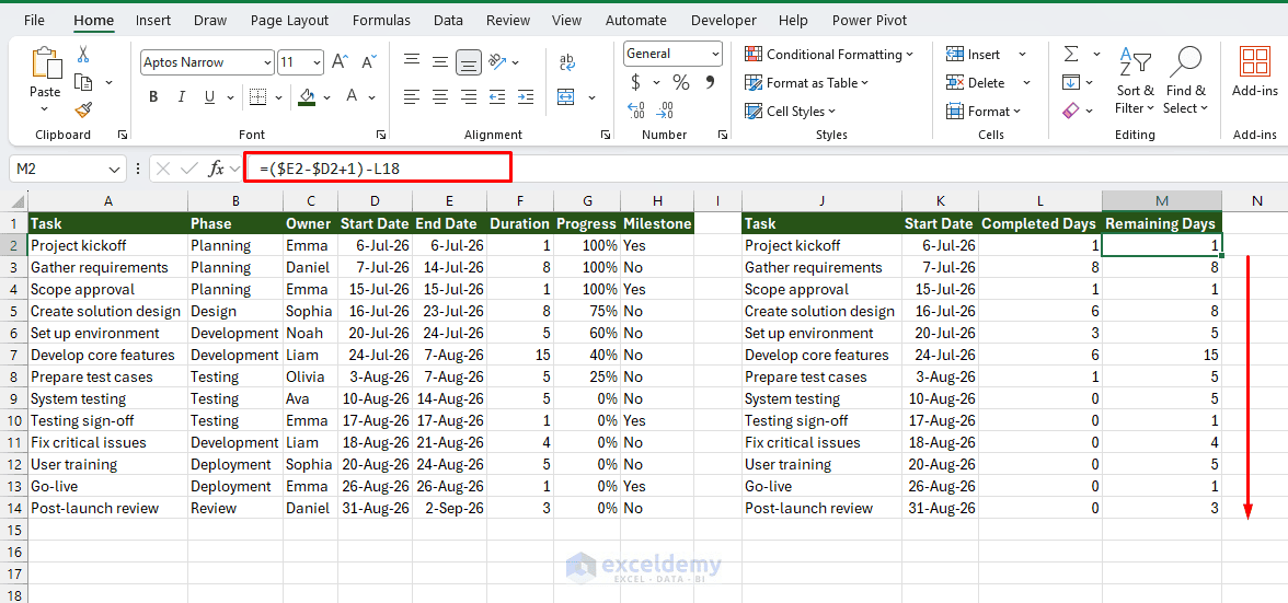
The three numerical series serve different purposes:
- Start Date moves each task bar to the correct position.
- Completed Days represents the completed portion.
- Remaining Days represents unfinished work.
Step 2: Insert the Chart and Select the Data Source
- Select the columns from the helper table.
- Go to the Insert tab >> select Column or Bar Chart >> select Stacked Bar.
- Excel will insert a stacked bar chart.
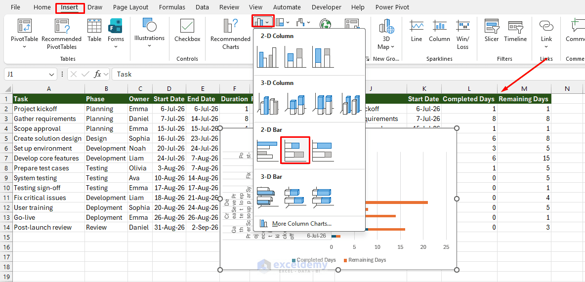
The task names should appear on the vertical axis. If Excel automatically adds unwanted data, right-click the chart, choose Select Data, and remove the unwanted series.
Add the Start Date Series Manually:
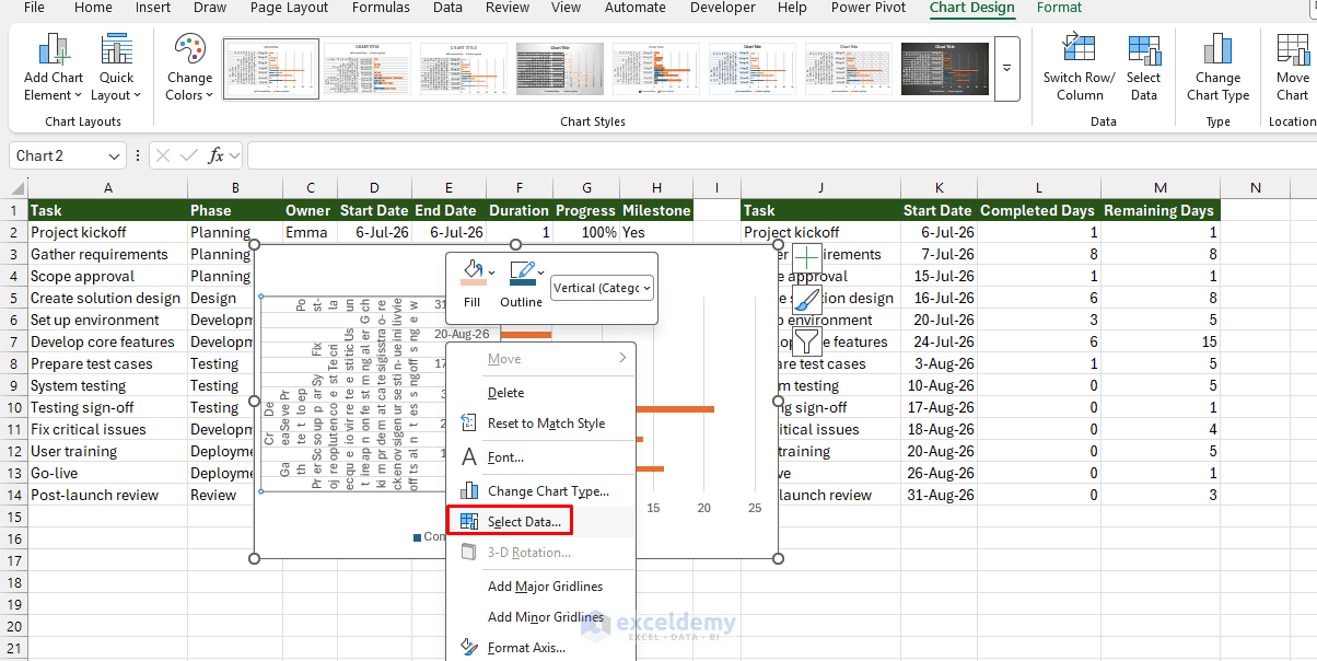
Excel may not correctly separate the multiple columns of data. You can correct this using the Select Data option.
- Right-click >> choose Select Data.
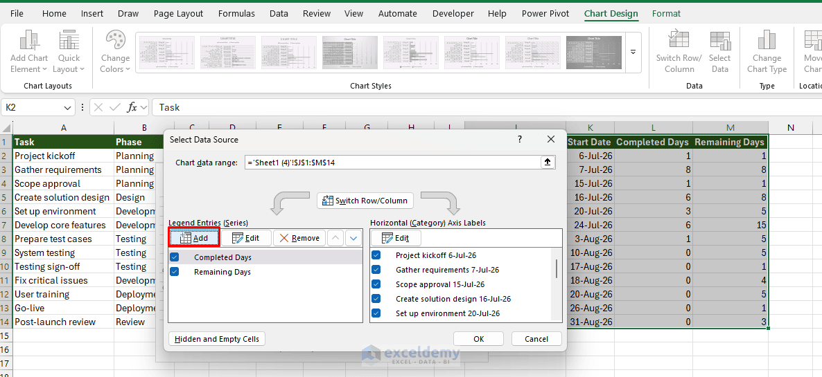
- Under Legend Entries (Series) >> click Add.
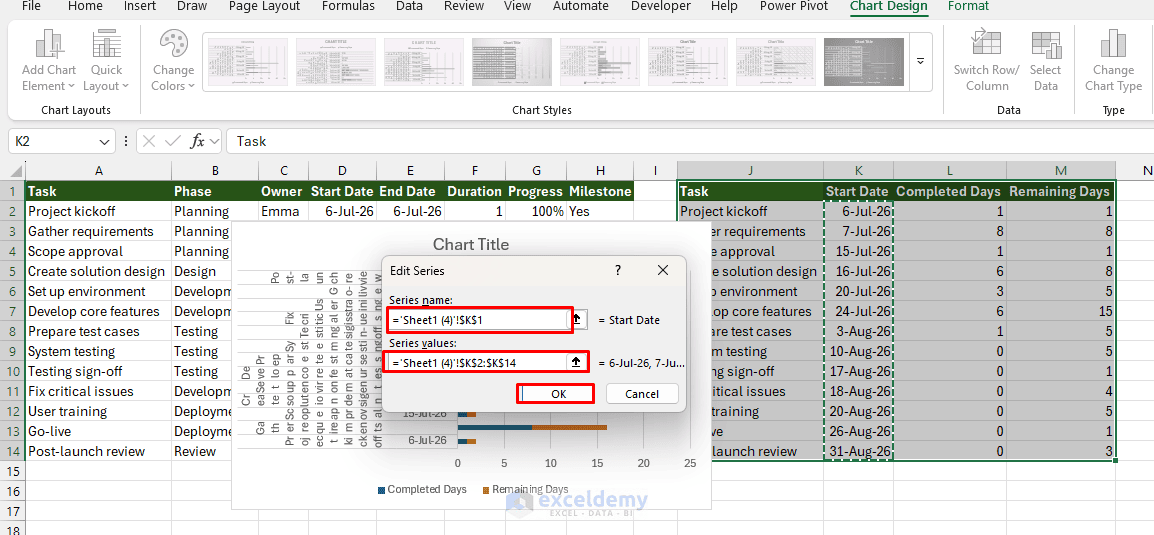
- For Series name, select: =$K$1
- For Series values, select: =$K$2:$K$14
- Click OK.
Insert the Completed Days and Remaining Days data series by following similar steps.
The series must appear in this order:
- Start Date
- Completed Days
- Remaining Days
Use the arrow buttons in the Select Data Source dialog box to rearrange them when necessary.
Add the Task Names as Axis Labels:
- In the Select Data Source dialog box >> select Horizontal (Category) Axis Labels.
- Click Edit >> select: =$J$2:$J$14
- Click OK.
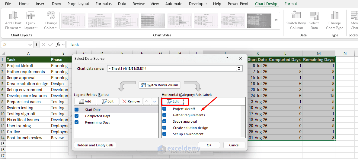
The task names should now appear without the start dates beside them.
Step 3: Hide the Start Date Series
The Start Date series is needed to position the bars correctly, but it should not be visible.
- Select the Start Date series in the chart.
- Right-click >> choose Format Data Series.
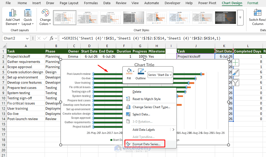
- Under Fill, select No Fill.
- Under Border, select No Line.
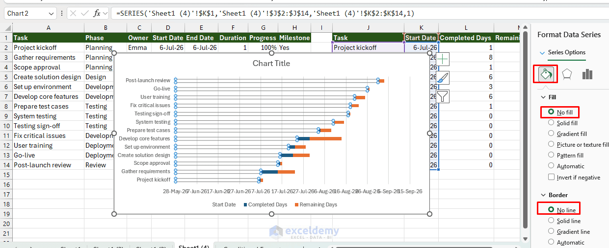
The completed and remaining portions will now appear to float at their actual project dates.
Step 4: Reverse the Task Order
Excel normally places the first task at the bottom of a bar chart.
- Right-click the vertical task axis >> choose Format Axis.
- Select Categories in reverse order.
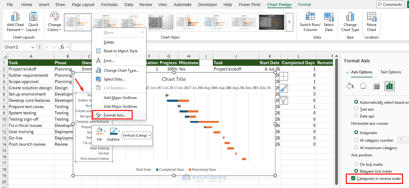
The first project task will move to the top.
Step 5: Format the Date Axis
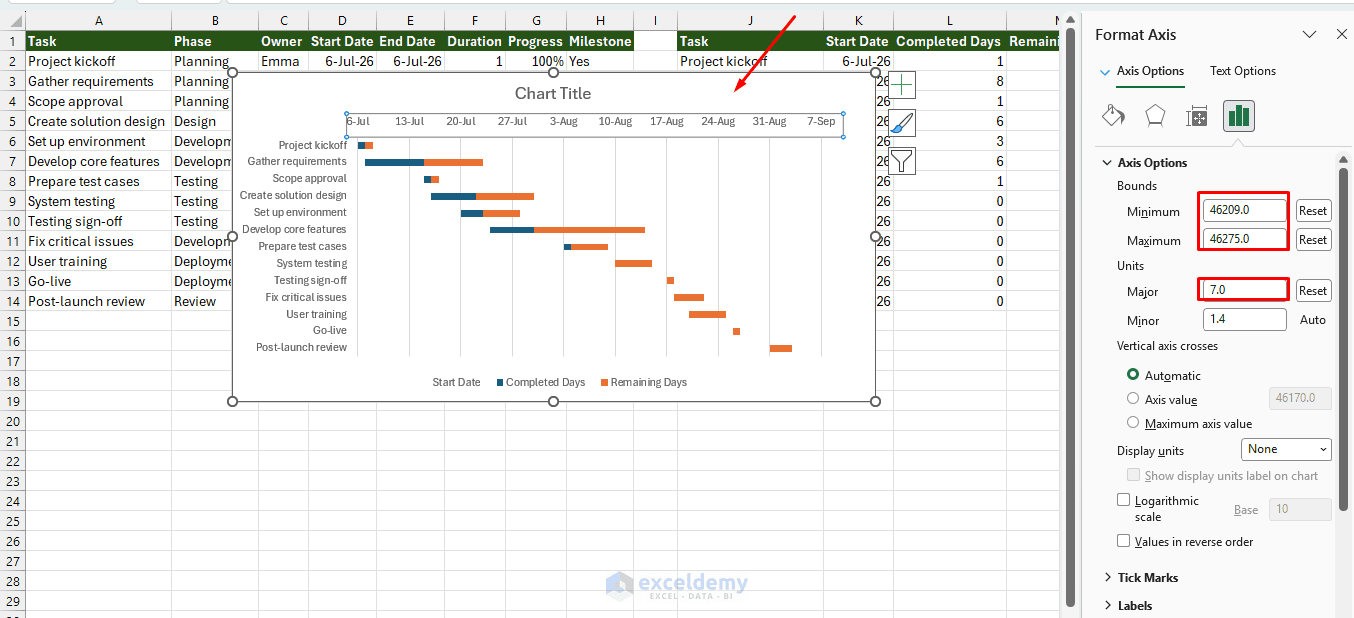
- Right-click the horizontal axis >> choose Format Axis.
- Under Bounds:
- Set the Minimum value to the first project date, such as: 6-Jul-2026 (46209).
- Set the Maximum value to a date shortly after the final project date, such as: 7-Sep-2026 (46275).
- Set the major units to 7 (for weekly gridlines) to control how often dates appear.
- Under Number, apply a date format such as: d-mmm.
Step 6: Improve the Chart
You can improve the chart by:
- Reducing the Gap Width between the bars.
- Giving completed and remaining work different fill colors.
- Removing unnecessary chart borders.
- Adding a chart title.
- Displaying data labels for completed or remaining days.
- Increasing the chart height so task names remain readable.
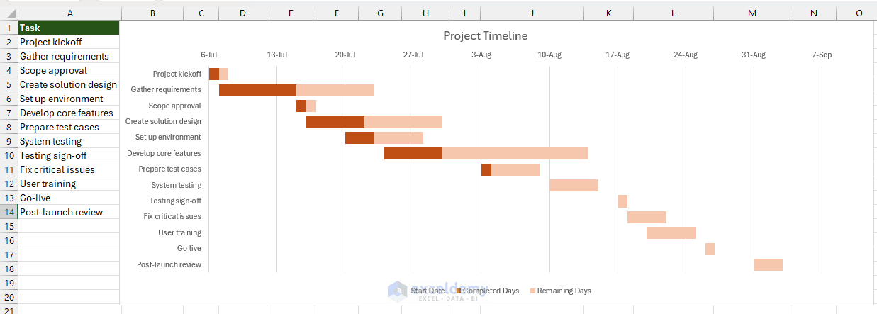
The finished Gantt chart shows the project schedule and the progress of every task.
Method 4: Build a Milestone Timeline with a Scatter Chart
A full Gantt chart may contain more detail than senior managers or clients need. A milestone timeline focuses only on important project events.
Step 1: Create the Milestone Table
Enter the milestone table in an unused section of the worksheet. Only include tasks where the Milestone column contains Yes. Alternating the position between 1 and -1 prevents the labels from overlapping. The positive and negative position values place the milestone labels above and below the timeline.
Step 2: Insert a Scatter Chart
- Select the Milestone Date and Position columns.
- Go to the Insert tab >> select Scatter Chart >> select Scatter with Only Markers.
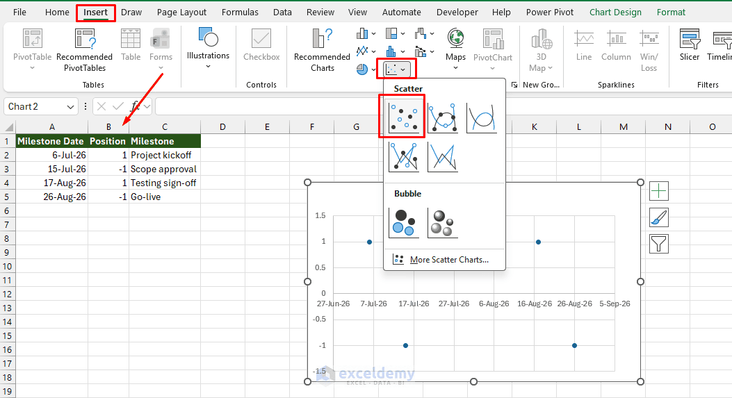
Excel will place the milestone dates along the horizontal axis.
Step 3: Add Milestone Names
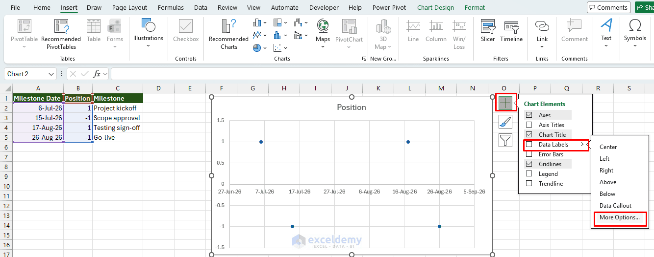
- Select the chart markers.
- Go to Chart Elements >> select Add Chart Element >> select Data Labels >> select More Data Label Options.
- In the Format Data Labels pane >> select Value From Cells.
- Select the milestone names from the helper table.
- Clear the checkboxes for:
- X Value
- Y Value
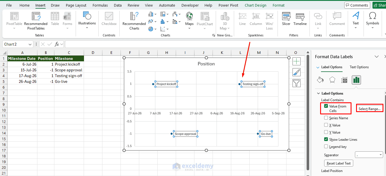
Only the milestone names should remain.
Step 4: Format the Vertical Axis
- Right-click the vertical axis and choose Format Axis.
- Set:
- Minimum: -1.5
- Maximum: 1.5
- Major: 0.5
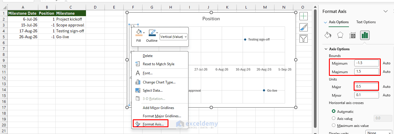
You can then hide the vertical axis, since the position values are only used to arrange the labels.
Step 5: Format the Horizontal Axis
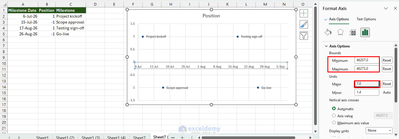
Format the horizontal axis as a date.
- Set the minimum date to the beginning of the project.
- Set the maximum date to the end of the project.
- Apply a format such as: d-mmm.
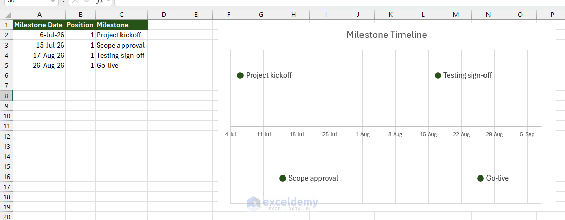
The result is a clean milestone timeline showing only important project dates.
Method 5: Create a Presentation Timeline with SmartArt
SmartArt is useful when you need a simple timeline for a presentation, project proposal, or status report.
Unlike the previous methods, SmartArt is not directly connected to the project data. You must update the timeline manually when milestone dates change.
Step 1: Insert the SmartArt Timeline
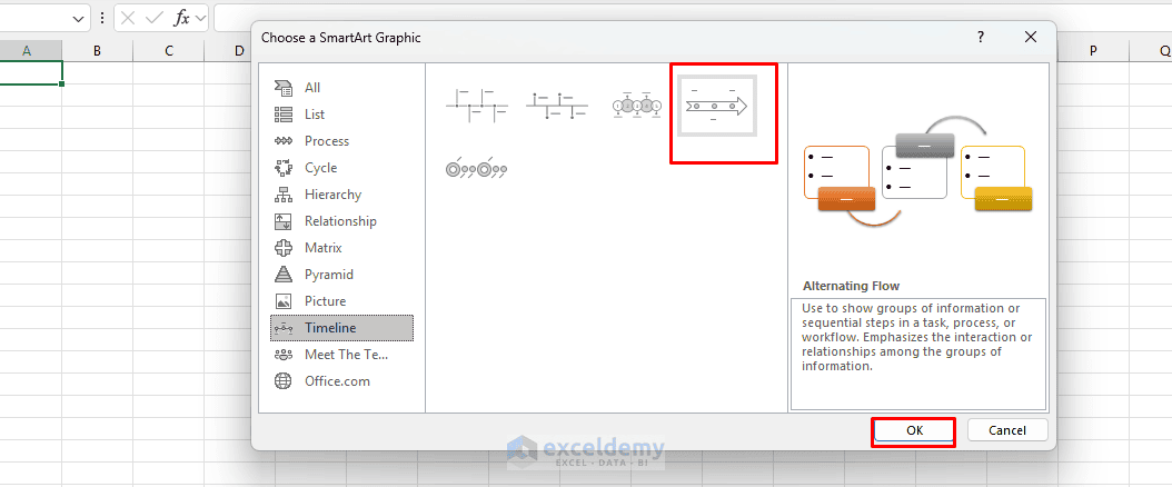
- Go to the Insert tab >> select Illustrations >> select SmartArt.
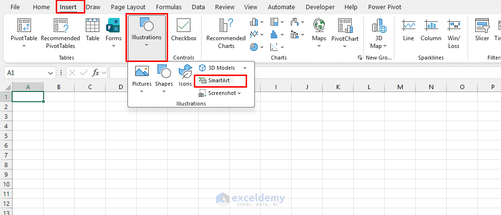
- Choose a layout such as Basic Timeline.
- Click OK.
Step 2: Enter the Milestones
Open the SmartArt text pane and enter the important project events.
- 6-Jul-26 – Project kickoff
- 15-Jul-26 – Scope approval
- 17-Aug-26 – Testing sign-off
- 26-Aug-26 – Go-live
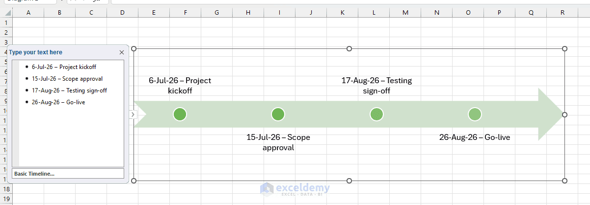
Each line creates another point on the timeline.
Step 3: Add or Remove Timeline Points
To add another milestone:
- Select a SmartArt shape.
- Go to the SmartArt Design tab >> select Add Shape >> select Add Shape After.
To remove a milestone, select the corresponding shape and press Delete.
Step 4: Format the Timeline
Use the SmartArt Design and Shape Format tabs to change:
- The SmartArt layout.
- Shape styles.
- Fonts and text sizes.
- Timeline direction.
- Colors.
- Shape sizes.
Keep the milestone descriptions brief so that the timeline remains readable.
SmartArt works best when you need to communicate four to eight important project events rather than every individual task.
Which Project Timeline Method Should You Use?
| Method | Best For | Main Advantage | Limitation |
| Formula-based grid | Small daily schedules | Simple and easy to build | Limited visual formatting |
| Conditional formatting | Dynamic project tracking | Updates automatically | Wide projects may require many columns |
| Stacked bar Gantt chart | Reports and dashboards | Professional chart-based view | Requires helper columns |
| Scatter milestone chart | Key events and deadlines | Clean executive-level view | Does not show detailed task durations |
| SmartArt timeline | Presentations and proposals | Fast and visually attractive | Must be updated manually |
Conclusion
You don't need specialized add-ins to create effective project timelines in Excel. Excel's formulas, conditional formatting, charts, and SmartArt provide enough flexibility to build both detailed project schedules and high-level management timelines without requiring any external tools. By combining these built-in features, you can create professional project timelines that remain flexible, scalable, and easy to maintain.
Get FREE Advanced Excel Exercises with Solutions!