


VLOOKUP has been one of Excel’s most popular lookup functions for decades. It was the go-to function for anyone who needed to search a spreadsheet and pull back a matching value. But it has several limitations: it searches only from left to right, depends on a fixed column number, returns only the first match, and uses approximate matching by default when the final argument is omitted. XLOOKUP, introduced in Excel 365 and Excel 2021, was built specifically to fix these problems. It can search in either direction, return multiple columns, provide a custom message when no result is found, perform wildcard searches, and search from the bottom of a dataset.
In this tutorial, we walk through 7 XLOOKUP tricks that make VLOOKUP obsolete. XLOOKUP offers greater flexibility, fewer errors, and advanced capabilities while being easier to use in most scenarios.
Quick Refresher: XLOOKUP Syntax
=XLOOKUP(lookup_value, lookup_array, return_array, [if_not_found], [match_mode], [search_mode])
Only the first three arguments are required. The last three are optional, and as you’ll see below, they’re where most of XLOOKUP’s power lives.
Trick 1: Look Left Without Rearranging Your Data
VLOOKUP can only search left-to-right; the column you’re searching must be to the left of the column you want returned. If your data isn’t arranged that way, you’re stuck rearranging columns or using INDEX/MATCH.
XLOOKUP removes this restriction entirely. The lookup array and return array are independent, so direction doesn’t matter.
Suppose you want to find an Order ID based on Revenue, but the Order ID is to the left of Revenue. VLOOKUP can’t do this without rearranging columns.
- Insert the following formula to get the Order ID:
=XLOOKUP(M2,J2:J121, A2:A121)
This searches for the Revenue value and returns the corresponding value from the Order ID column, regardless of which column comes first. This flexibility eliminates the need to rearrange tables or use workarounds like INDEX/MATCH.
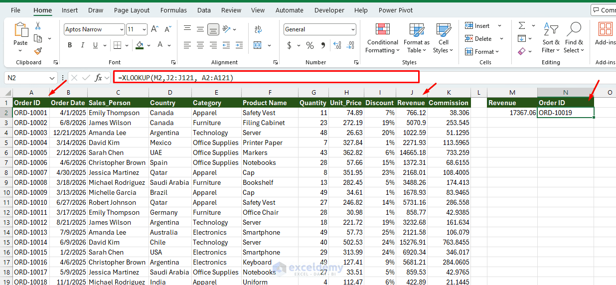
This is one of the most important differences between XLOOKUP and VLOOKUP. XLOOKUP can return information from either side of the lookup column, while VLOOKUP requires the lookup column to be the leftmost column of its table range.
Why it matters: You never have to restructure a spreadsheet just to satisfy a formula’s directional requirement.
Trick 2: Return Multiple Columns in One Formula
With VLOOKUP, returning several pieces of information means writing three separate VLOOKUP formulas, each with a different column index number.
XLOOKUP lets you return an entire range as the return array, spilling the results across multiple cells with a single formula.
Suppose you want to return the product, quantity, unit, and revenue based on an Order ID — something that would require several separate VLOOKUP formulas.
=XLOOKUP(M6, A2:A121,F2:J121)
This single formula spills all values into adjacent cells starting at the formula’s location; there’s no need to write it three times. Do not enter anything in the cells to the right of N6. Excel needs those cells to be empty so that the results can spill across them.
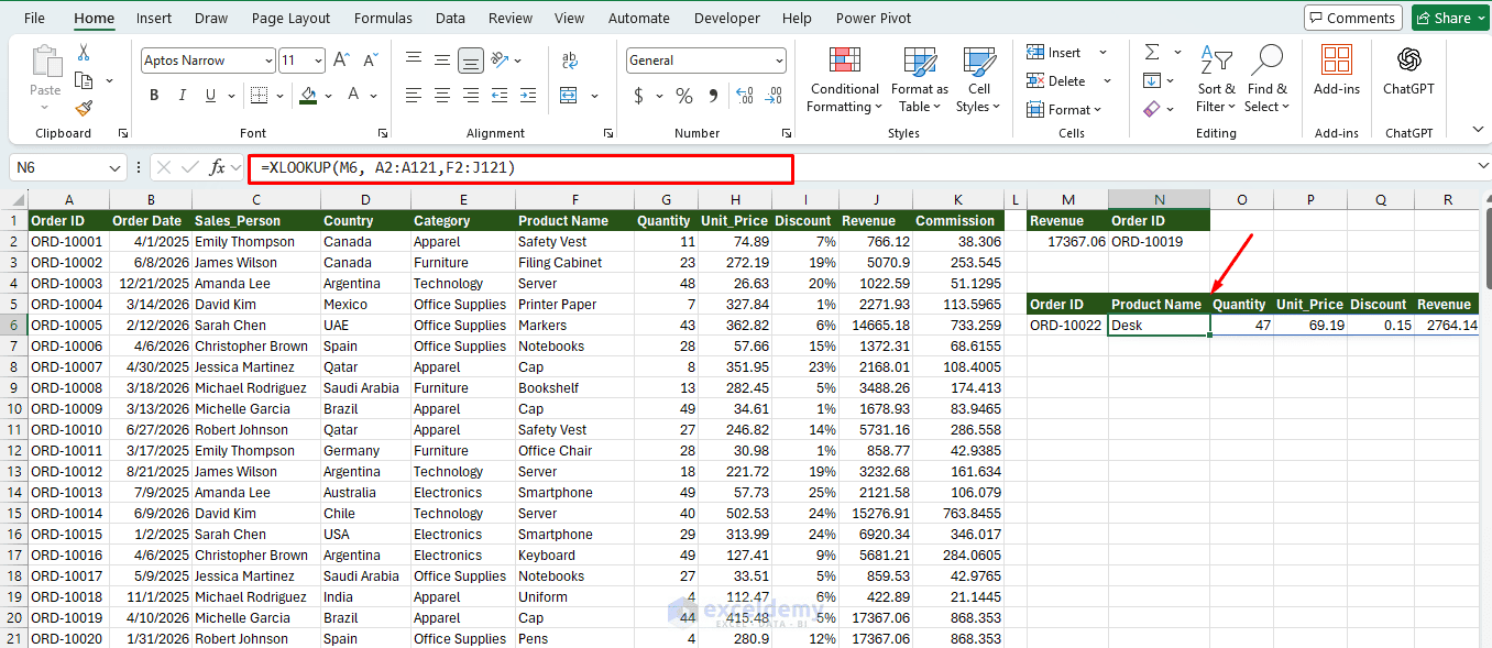
A single XLOOKUP formula can return multiple items from the matching row when its return array contains several columns.
Why it matters: One formula, one point of maintenance. If you need to insert a new field between F and J, you don’t need to touch the formula at all — the spill range adjusts automatically.
Trick 3: Say Goodbye to #N/A Errors with Built-In Fallbacks
VLOOKUP requires wrapping the whole function in IFERROR or IFNA to handle missing matches gracefully:
=IFERROR(VLOOKUP(F2, A:B, 2, FALSE), "Not Found")
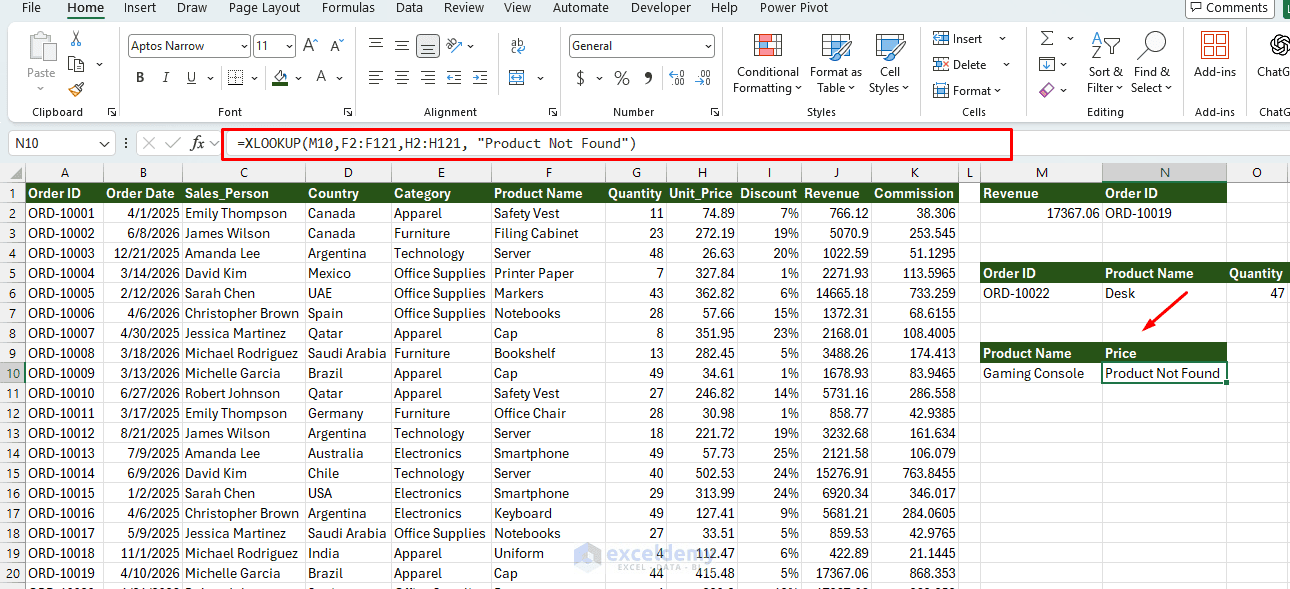
XLOOKUP builds this directly into its syntax with the fourth argument, if_not_found. If you’re looking up a product that doesn’t exist in your list, instead of a jarring #N/A error, the cell will simply display “Not Found” (or whatever text, number, or blank value you specify).
=XLOOKUP(M10,F2:F121,H2:H121, "Product Not Found")
This formula searches for the product in the product column; if it isn’t found, it displays customized text rather than an error.
Why it matters: Shorter formulas, easier auditing, and no separate error-handling layer to remember.
Trick 4: Use Approximate Match Without Sorting Data First
VLOOKUP’s approximate match mode (the fourth argument set to TRUE or omitted) requires your lookup column to be sorted in ascending order; otherwise, results are unreliable.
XLOOKUP’s match_mode argument supports approximate matches — both “next larger” and “next smaller” — without requiring sorted data.
Approximate matching is useful when values fall into ranges, such as commission rates, tax bands, shipping charges, performance ratings, quantity discounts, and similar tiered structures.
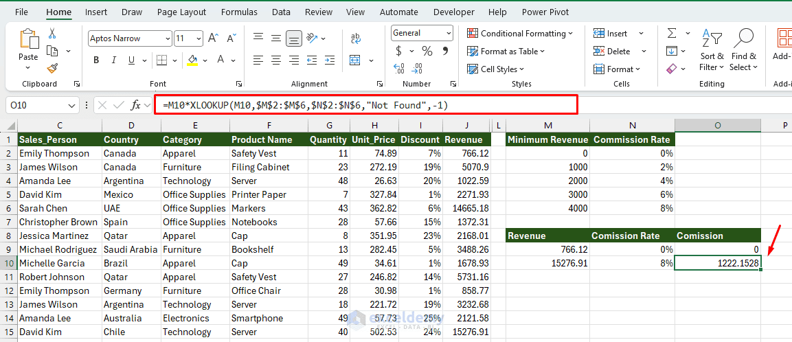
Imagine you have commission tiers based on sales thresholds, and you want to find which tier a given sales figure falls into, even if the threshold table isn’t sorted.
Minimum Revenue Commission Rate
0 0%
1000 2%
2000 4%
3000 6%
4000 8%
Make sure the minimum revenue values are arranged from smallest to largest.
=XLOOKUP(M10,$M$2:$M$6,$N$2:$N$6,"Not Found",-1)
Setting match_mode to -1 returns the next smallest match if an exact one isn’t found — perfect for tiered pricing, grading scales, or shipping rate brackets.
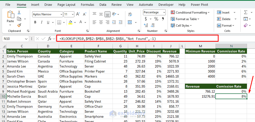
The -1 match mode means:
- Look for an exact match.
- If an exact match does not exist, return the result associated with the next smaller value.
The formula can also be used to calculate the actual commission:
=M10*XLOOKUP(M10,$M$2:$M$6,$N$2:$N$6,"Not Found",-1)
XLOOKUP uses the following values for its match modes:
- 0 = Exact match
- -1 = Exact match or next smaller value
- 1 = Exact match or next larger value
- 2 = Wildcard match
These match modes are built directly into the function.
Why it matters: You can keep your reference tables in whatever order makes sense to you, rather than reorganizing them purely to satisfy a lookup formula.
Trick 5: Search From the Bottom Up
VLOOKUP always returns the first match it finds, scanning top to bottom. If your data is organized so that the most recent or most relevant entry is at the bottom — like a transaction log — VLOOKUP will return outdated results.
XLOOKUP’s sixth argument, search_mode, lets you flip the search direction. Setting it to -1 searches from the last row to the first.
Real datasets often contain repeated values. An employee, customer, or product may appear across several transactions. In such cases, you may need the most recent or last matching record.
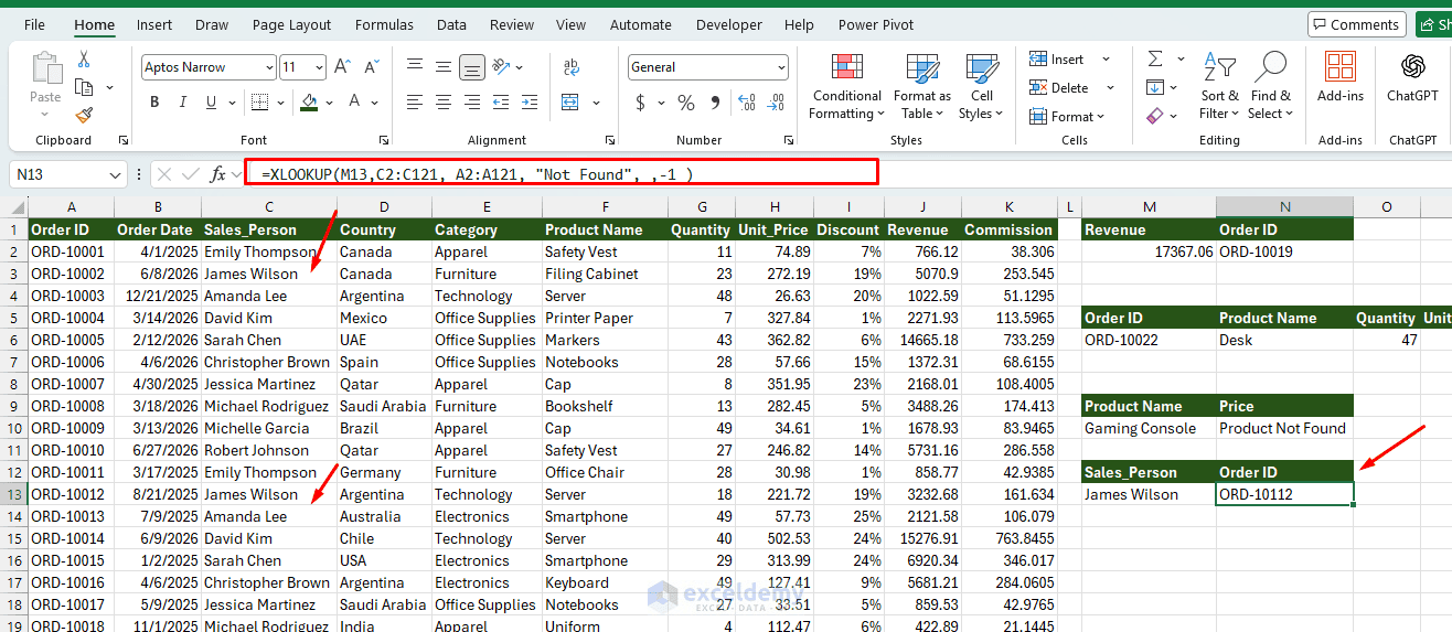
- Find the last sale for a particular salesperson:
=XLOOKUP(M13,C2:C121, A2:A121, "Not Found", ,-1 )
This salesperson has multiple records, but XLOOKUP finds the last occurrence and returns the most recent Order ID.
The search mode options are:
- 1 = Search from first to last
- -1 = Search from last to first
- 2 = Binary search on ascending data
- -2 = Binary search on descending data
Search mode -1 is particularly useful for finding:
- The latest transaction for a customer
- The most recent status update
- The last price recorded for a product
- The newest payment from an account
- The latest attendance record
Reverse searching is a built-in XLOOKUP feature and does not require rearranging the original data.
Why it matters: No need to sort data, add helper columns, or use array formulas just to find the most recent match.
Trick 6: Combine XLOOKUP with Wildcards for Flexible Text Matching
VLOOKUP supports wildcards, but only in exact match mode, and the syntax can get finicky. XLOOKUP handles wildcard matching cleanly through its match_mode argument by setting it to 2.
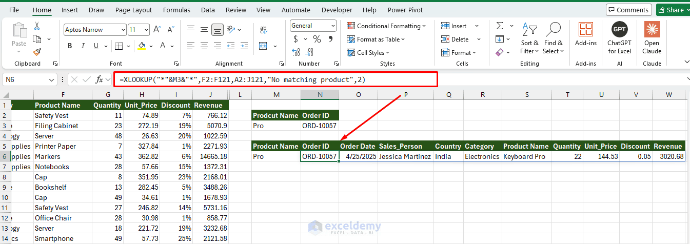
Sometimes you know only part of a product name. For example, you may remember that the name contains “Pro,” but not whether it is “Keyboard Pro” or “Monitor Pro.”
=XLOOKUP("*"&M3&"*",F2:F121,A2:A121,"No matching product",2)
This searches the product column for any entry containing “Pro” and returns the corresponding Order ID. The formula finds the first product containing the word “Pro,” which is Laptop Pro.
The two asterisks are wildcard characters: *Pro*. This pattern means that any number of characters can appear before or after the word “Pro.” The final argument, 2, tells XLOOKUP to use wildcard matching.
You can also return the complete matching record:
=XLOOKUP("*"&M3&"*",F2:F121,A2:J121,"No matching product",2)
Useful wildcard characters include:
*— Matches any number of characters.?— Matches exactly one character.~— Treats the next wildcard character as a literal character.
For example, the following pattern finds a five-letter product beginning with “M”:
=M????
A corresponding formula could be:
=XLOOKUP("M????",F2:F121,A2:J121,"No match",2)
Why it matters: Useful for messy, real-world data — partial product codes, inconsistent name spellings, or searching within longer text strings.
Trick 7: Nest XLOOKUP for Two-Way (Row + Column) Lookups
A two-way lookup finds a value based on both a row heading and a column heading. VLOOKUP alone can’t perform a true two-dimensional lookup — matching both a row and a column simultaneously — without pairing it with MATCH inside the column-index argument, which gets confusing fast.
XLOOKUP handles this cleanly by nesting one XLOOKUP inside another: the inner XLOOKUP finds the correct column, and the outer XLOOKUP finds the correct row within it.
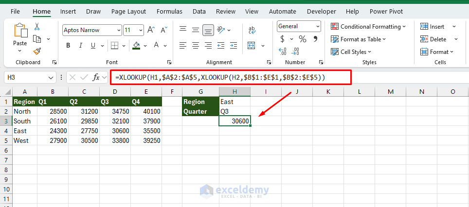
Suppose you have a table where rows are regions and columns are quarterly sales figures, and you want the sales number for a specific region and a specific quarter.
=XLOOKUP(H1,$A$2:$A$5,XLOOKUP(H2,$B$1:$E$1,$B$2:$E$5))
Here, H1 contains the region and H2 contains the quarter. The inner XLOOKUP finds the correct quarter column; the outer XLOOKUP finds the correct row for that region within it.
To display a custom message when either entry is invalid, wrap the formula in IFERROR:
=IFERROR(XLOOKUP(H1,$A$2:$A$5,XLOOKUP(H2,$B$1:$E$1,$B$2:$E$5)),"Region or quarter not found")
Nested XLOOKUP formulas can replace a combination of INDEX and MATCH, or a combination of VLOOKUP and HLOOKUP. Microsoft also documents nested XLOOKUP as a supported method for performing vertical and horizontal matching in the same formula.
Why it matters: This replaces the classic INDEX/MATCH/MATCH combination with a more readable, self-contained formula.
XLOOKUP vs. VLOOKUP
| Feature | VLOOKUP | XLOOKUP |
| Exact match by default | No | Yes |
| Lookup to the left | No | Yes |
| Return multiple columns | Not with one formula | Yes |
| Built-in not-found message | No | Yes |
| Search from last to first | No | Yes |
| Uses fixed column numbers | Yes | No |
| Wildcard matching | Yes | Yes |
| Vertical lookup | Yes | Yes |
| Horizontal lookup | No | Yes |
| Two-way lookup | Requires additional functions | Nested XLOOKUP |
| Approximate match options | Limited | More flexible |
Common Mistakes to Avoid
- Forgetting XLOOKUP requires Excel 365 or 2021: If you share a file with someone using Excel 2019, the formula will show a #NAME? error.
- Mixing up match_mode values: Remember: 0 = exact match, -1 = exact or next smallest, 1 = exact or next largest, 2 = wildcard match.
- Assuming search_mode changes what’s matched: It only changes search direction (top-down vs. bottom-up), not the matching logic itself.
- Overusing wildcards on large datasets: Wildcard searches are slower than exact matches, so use them selectively on smaller ranges when possible.
- Not locking reference ranges with $ when copying formulas across cells: This is the same rule that applied to VLOOKUP, and it still applies here.
Conclusion
These are the 7 XLOOKUP tricks that make VLOOKUP obsolete. XLOOKUP isn’t just a replacement for VLOOKUP — it’s a rethinking of how lookups should work in Excel. Bidirectional searching, built-in error handling, multi-column returns, and flexible matching modes solve problems that used to require nested formulas or helper columns. VLOOKUP may remain useful when maintaining older workbooks, but for modern Excel projects, XLOOKUP provides clearer, safer, and more flexible formulas. Once you get comfortable with these seven tricks, going back to VLOOKUP will feel like using a flip phone after switching to a smartphone.
Get FREE Advanced Excel Exercises with Solutions!


Thank you so much.
Hello Mohammad,
You are most welcome. Thanks for your feedback and appreciation.
Keep exploring Excel with ExcelDemy!
Regards,
ExcelDemy