Use of CHOOSE Function with Array in Excel: 7 Simple Examples

Example 1 – Return a Single Value Using the CHOOSE Function with an Array

Steps:

• Input the array search number in cell E4.
• Use the following formula in cell E5:

• Press the Enter key.

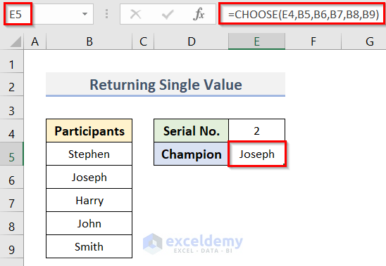
Cell E4 refers to the position of the value to return. Cell E4 is the index_num. Besides, the cells B5, B6, B7, B8, and B9 are the values from which the function will choose the Champion. We inserted the cell names separately instead of a range because the CHOOSE function does not support a range.

Example 2 – Apply the CHOOSE Function with an Array to Return Multiple Values in Excel

Steps:

• Select cell B12.
• To get the values in a row, enter the formula below in the cell:

• Press the Enter key.
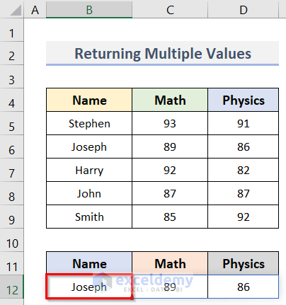
• Get the values in the range B12:D12 (see the picture below).

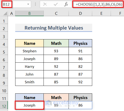
In the formula, the cells B6, C6, and D6 denote the values to be returned. Again, {1,2,3} array refers to the positions of the values. So, {1,2,3} array is the index_num in this formula.

• By applying this formula, we get the result in an array format.
• The other two values will automatically be selected (see screenshot).
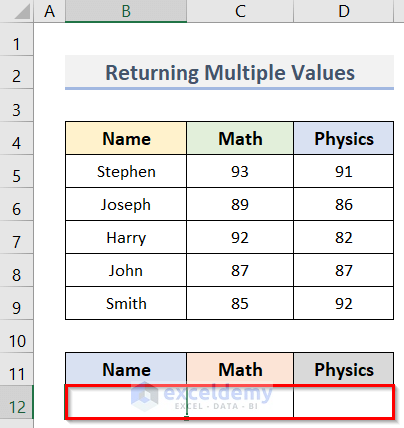
• To delete the entire array, you must select a single cell (cell B12 in our case).

• Press the Delete button on the keyboard.
• All three values in the array will be removed at once.

Example 3 – Excel CHOOSE Function with an Array to Find Values Depending on Specific Conditions

Steps:

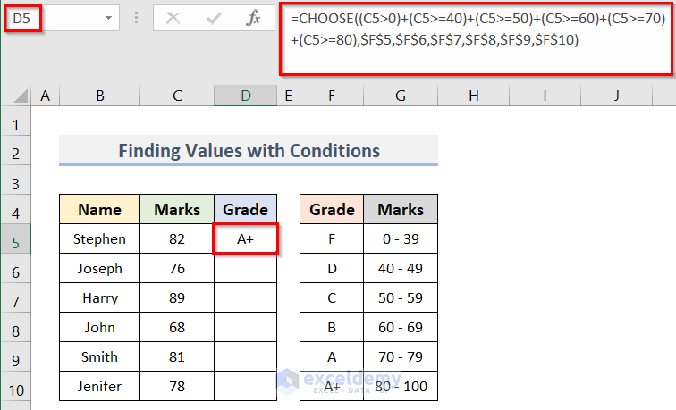
• Insert the formula below in cell (D5) to find the Grade of Stephen:

• Press the Enter key on the keyboard.

How Does the Formula Work?

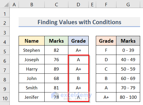
• Put the cursor in the bottom-right corner of cell D5.
• You will see a plus sign (+) there.

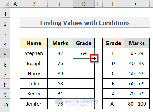
• Double-click on the plus sign.

Example 4 – Use an Array in the CHOOSE Function for Calculations

Steps:

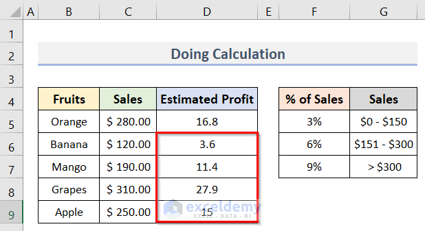
• We’ll calculate the Estimated Profit of Orange.
• Go to cell D5.
• Use the following formula in the cell to calculate the Estimated Profit:

• After pressing the Enter key, you will find the Estimated Profit of Orange in cell D5.

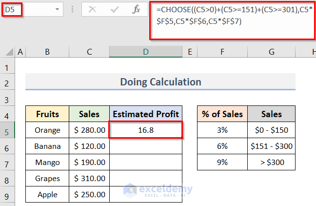
This formula works in the same way as the previous method. It multiplies the % of Sales ($F$5, $F$6 & $F$7) with the Sales (C5) based on their values ((C5>0)+(C5>=151)+(C5>=301)).

• Double-click on the Fill Handle to auto-fill the rest of the cells (D6:D9).

Example 5 – Apply the CHOOSE Function with an Array for Left VLOOKUP

Steps:

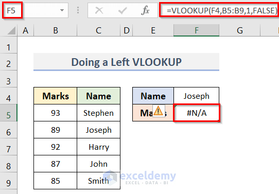
• We’ll try to get the Marks of Joseph with the following formula:

• We get an #N/A error (see screenshot). The VLOOKUP function can only search for the value in the left-most column.

• We’ll use the CHOOSE function in the VLOOKUP function to solve this:

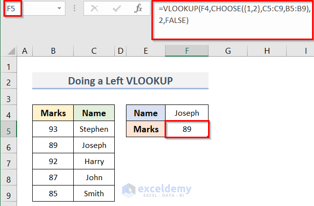
How Does the Formula Work?

Example 6 – Combination of Excel SUM and CHOOSE Functions with an Array

Steps:

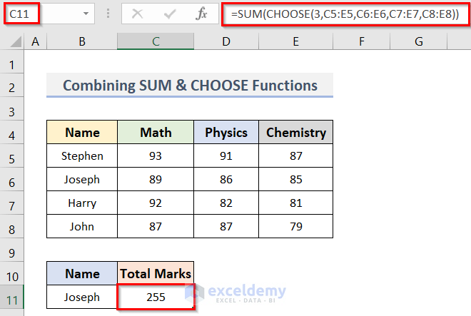
• To get the Total Marks of Joseph, insert the formula below:

• Press the Enter key to get the output (see screenshot).

How Does the Formula Work?

Example 7 – Assign the CHOOSE Function with Array to Return a Cell Reference

Steps:

• To get the fruit of ID = 2, insert the formula below in cell E5:

• Press Enter.

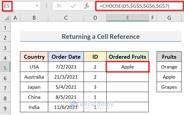
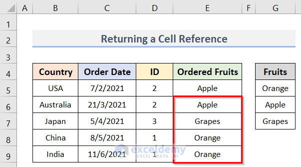
In the formula, cell D5 refers to the position number 2. The formula returns the second fruit (Apple) from the list ($G$5,$G$6,$G$7).

• Double-click on the plus sign to auto-fill the rest of the cells (see screenshot).

Things to Remember

• You can’t use more than 254 values in this function.
• When the index_num is less than 1 or greater than 254, the function returns the #VALUE! error.
• If the entered index_num is a fraction, the function rounds it to the lower integer.

Download the Practice Workbook

Related Articles

• How to Apply CHOOSE Function to Create Drop-Down List in Excel
• How to Use CHOOSE Function in Excel for Scenarios
• How to Use CHOOSE Function to Perform IF Condition in Excel

<< Go Back to Excel CHOOSE Function | Excel Functions | Learn Excel