Method 1 – Getting Random Integers
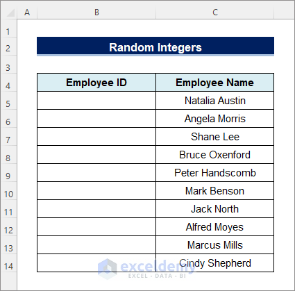
Look at the data set below. We have the names of 10 employees of Sunshine Group.
- Provide each employee with an employee ID between 101 and 110. We can provide that using the RANDBETWEEN function of Excel. Enter this formula into each of the cells.
=RANDBETWEEN(101,110)
The RANDBETWEEN(101,110) syntax returns a random integer between 101 and 110.
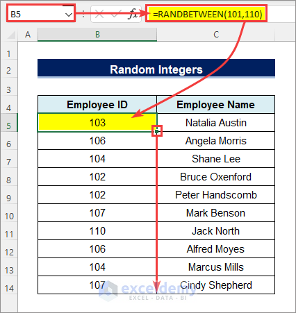
We inserted an ID between 101 to 110 for each of the employees.
Note: There is a problem here. We want the employee IDs to be unique, right? That means each of the 10 employees will have a unique employee ID between 101 and 110.
Using only the RANDBETWEEN function 10 times does not give any guarantee to provide 10 unique numbers. In the image above, 106, 104, 102, and 107 have been repeated. To get the desired value, follow the below steps. Use the combined formula of applying INDEX, FILTER, COUNTIF, RANDBETWEEN, ROW, and ROWS functions to get a unique employee ID for each employee randomly.
- Fill up the first cell using a simple RANDBETWEEN function.
=RANDBETWEEN(101,110)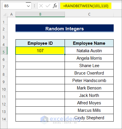
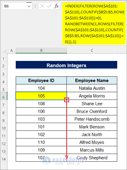
- Insert this complex formula in the 2nd cell.
=INDEX(FILTER(ROW($A$101:$A$110),COUNTIF($B$5:B5,ROW($A$101:$A$110))=0),RANDBETWEEN(1,ROWS(FILTER(ROW($A$101:$A$110),COUNTIF($B$5:B5,ROW($A$101:$A$110))=0))),1)Formula Explanation
- We used ROW(A101:A110) because we want random numbers between 101 and 110. If you want random numbers between 101 to 200, use ROW(A101:A200) or ROW(B101:B200), and so on.
- B5 cell within the COUNTIF function is the first cell reference where I manually inserted a number using a simple RANDBETWEEN You use your one.
- Double-click on the Fill Handle. You will find all the cells filled with unique random numbers from 101 to 110, like this:
Note: The FILTER function is available in only Office 365. So, you cannot use this formula unless you are in Office 365.
Method 2 – Getting Random Dates
Get any random date between two dates using the RANDBETWEEN function. Put two dates in place of the bottom and top arguments instead of numbers.
- Look at the data set below. The names of 10 candidates selected for an interview in the Sunshine Group.
- Enter random dates for their interviews in September 2021. That means the dates need to be between 1-September-2021 and 30-September-2021.
The formula will be:
=RANDBETWEEN(DATE(2021,9,1),DATE(2021,9,30))
Formula Explanation
- DATE(2021,9,1) and DATE(2021,9,30) return the bottom and top values, on 1-Sep-2021 and 30-Sep-2021. See the DATE function for details.
- RANDBETWEEN(DATE(2021,9,1),DATE(2021,9,30)) returns a random date between these two dates, including these two.
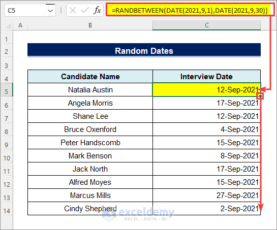
We got a random date for each of the candidates.
Note: We have the same problem as above. Some dates have been repeated. Like 12-Sep-2021 and 17-Sep-2021.
We want a unique date for each of the candidates.
We will accomplish this using a combination of Excel’s INDEX, FILTER, COUNTIF, RANDBETWEEN, SEQUENCE, ROWS, and DATE functions. The SEQUENCE function is only available in Office 365. Follow the below steps.
- Fill up the first cell with a simple RANDBETWEEN function.
=RANDBETWEEN(DATE(2021,9,1),DATE(2021,9,30))
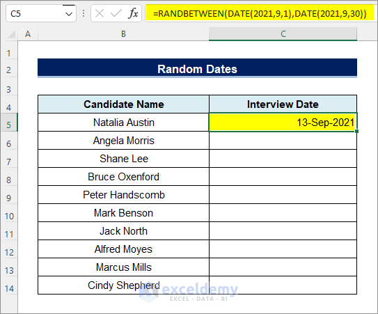
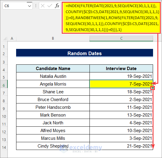
- Insert this complex formula in the 2nd cell.
=INDEX(FILTER(DATE(2021,9,SEQUENCE(30,1,1,1)),COUNTIF($C$4:C4,DATE(2021,9,SEQUENCE(30,1,1,1)))=0),RANDBETWEEN(1,ROWS(FILTER(DATE(2021,9,SEQUENCE(30,1,1,1)),COUNTIF($C$4:C4,DATE(2021,9,SEQUENCE(30,1,1,1)))=0))),1)
Formula Explanation
- Within SEQUENCE(30,1,1,1), 30 is the total number of dates within the interval. We have 1-sep to 30-Sep, a total of 30 days. Use your one.
- The third argument 1 within SEQUENCE(30,1,1,1) denotes the starting day of your interval. If you start on 15 September, use SEQUENCE(30,1,15,1).
- Within the DATE function, 2021 and 9 denote the year and month of the starting date. If you start in February 2022, use DATE(2022,2,…)
- C5 within the COUNTIF function denotes the first cell reference where I manually inserted a date.
- Double-click on the Fill Handle. You will see all the cells filled with unique dates from 1-Sep-2021 to 30-Sep-2021.
Method 3 – Selecting Random Data from a Table
We have a data set of the names and joining dates of 10 employees of the Sunshine Group.
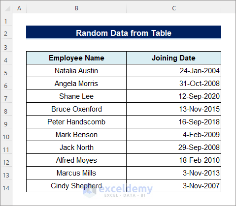
The company chief has decided to randomly throw a surprise party on the joining date of any employee.
Use this formula:
=INDEX(B5:C14,RANDBETWEEN(1,10),2)
Formula Explanation
- RANDBETWEEN(1,10) returns a random integer between 1 to 10. We used 1 to 10 because we have a total of 10 employees.
- INDEX(B5:C14,RANDBETWEEN(1,10),2) returns the cell content of the cell with the random row number and column number 2 (“Joining Date“) from the range B5:C14.
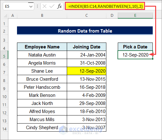
- We selected a date randomly from the table.
Method 4 – Dividing into Groups Using the RANDBETWEEN Function
Look at the data set below. We have a list of 12 countries qualified for the upcoming ICC Cricket World Cup in 2023.
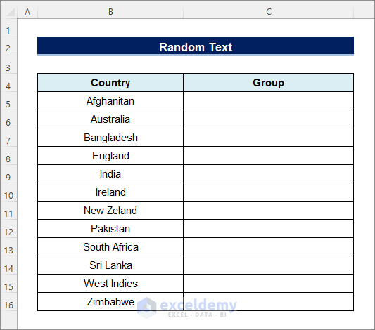
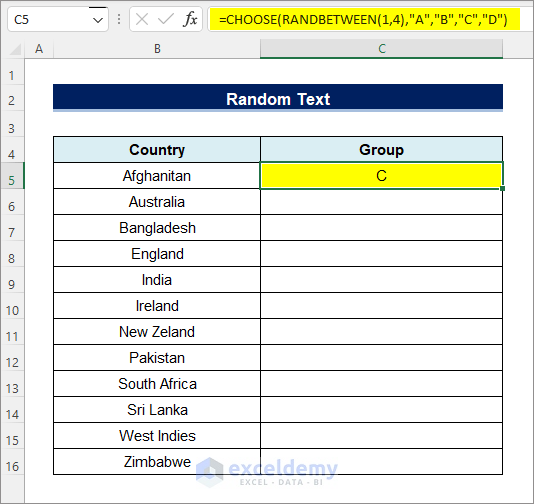
- Divide the teams into four groups, A, B, C, and D. You can use the CHOOSE function of Excel in combination with the RANDBETWEEN function to accomplish this.
=CHOOSE(RANDBETWEEN(1,4),"A","B","C","D")
Formula Explanation
- RANDBETWEEN(1,4) returns an integer between 1 and 4. We have taken 1 to 4 because there are 4 groups.
- CHOOSE(RANDBETWEEN(1,4),”A”,”B”,”C”,”D”) assigns one group to each of the teams based on the result of the RANDBETWEEN function.
We divided the teams into four groups.
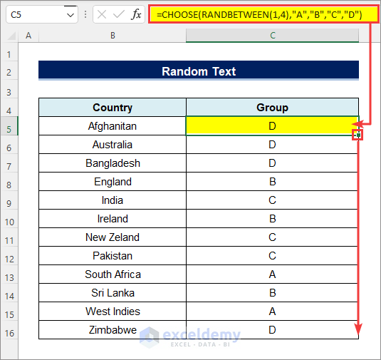
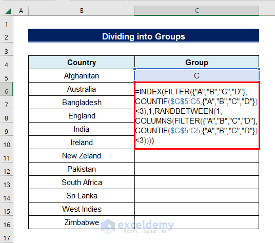
You will find there is a problem too. We want all the groups to have an equal number of teams, 3 in this case. But here we have got 4 teams in group D and 2 teams in group A. We do not want this. But no worries. We will solve this too. Follow the below steps.
- The first cell randomly has the CHOOSE function.
- Insert this complex formula in the 2nd (C6) cell.
=INDEX(FILTER({"A","B","C","D"},COUNTIF($C$5:C5,{"A","B","C","D"})<3),1,RANDBETWEEN(1,COLUMNS(FILTER({"A","B","C","D"},COUNTIF($C$5:C5,{"A","B","C","D"})<3))))
Formula Explanation
- {“A”,”B”,”C”,”D”} are the names of my groups. Use anything according to your wish.
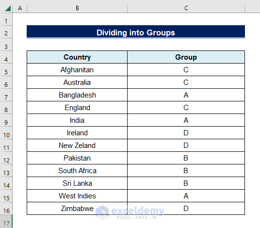
- We used COUNTIF($C$5:C5,{“A,” “B,” “C,” “D”})<3) because we want each group to have 3 teams. You use it accordingly.
- Within the COUNTIF function, C5 is the cell reference of the first cell where the group was manually inserted. You use your one.
- Double-click on the Fill Handle. Get all the cells filled with the groups, each group having 3 teams.
- Use this formula anywhere other than Office 365 because the FILTER function is only available in Office 365.
Method 5 – Using RANDBETWEEN Function for Decimals
The RANDBETWEEN function returns integer outputs only. Combine it with the RAND function to generate random decimal numbers between two specified numbers.
- Apply the formula in cell C5 and drag the Fill Handle icon below.
=RANDBETWEEN(101,110-1)+RAND()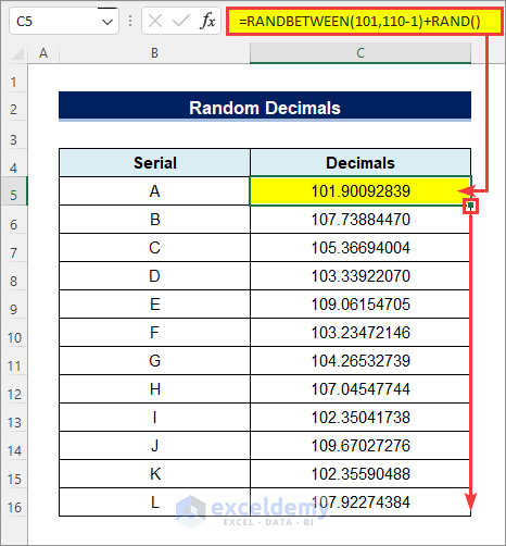
- Need to subtract 1 from the top argument to keep the generated number within the specified limits.
Limitations of Excel RANDBETWEEN Function
The output of the RANDBETWEEN function changes each time any other cell in the workbook or worksheet is changed. This cell may be connected to the function or not.
- Turn the RANDBETWEEN outputs into normal text values before going to another task.
- Select all the RANDBETWEEN
- Press Ctrl + C on your keyboard.
- Right-click on your mouse. From Paste Options, select

- Find all the RANDBETWEEN outputs converted into text values.
Common Errors with Excel RANDBETWEEN Function
| Error | When They Show |
|---|---|
| #NUM! | Shows when the bottom argument is less than the top argument. |
| #VALUE! | Shows when any argument is of the wrong data type. For example, when the top or bottom arguments are text values instead of numbers. |
Download Practice Workbook
<< Go Back to Excel Functions | Learn Excel
Get FREE Advanced Excel Exercises with Solutions!
