Introduction to the DATE Function
- Function Objective:
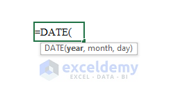
The DATE function creates a date from numeric values in the arguments.
- Syntax:
=DATE(year,month,day)- Arguments Explanation:
| ARGUMENT | REQUIRED/OPTIONAL | EXPLANATION |
| year | Required | The numeric value of year. |
| month | Required | The numeric value of month. |
| day | Required | The numeric value of day. |
- Return Parameter:
A date containing year, month, and day.
- Version:
The DATE function has been introduced in Excel 2007 and is available for all versions after that.
The DATE Function with Number in an Argument
Steps:
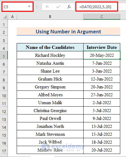
- Enter the number representing the year, month, and day in the arguments of the DATE function. The corresponding date will appear in the cell.
- Enter the following formula in cell C5:
=DATE(2022,5,20)- The formula gives the output date 20-May-2022. I have included more dates similarly.
The DATE Function with Cell Reference in an Argument
Steps:
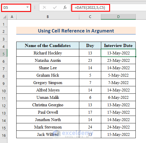
- Enter the following formula in cell D5:
=DATE(2022,5,C5)The formula takes the value of Cell C5 as the Day argument.
- We can see the corresponding date in Cell D5. I have included more dates in the sheet.
The DATE Function with Arrays
Steps:
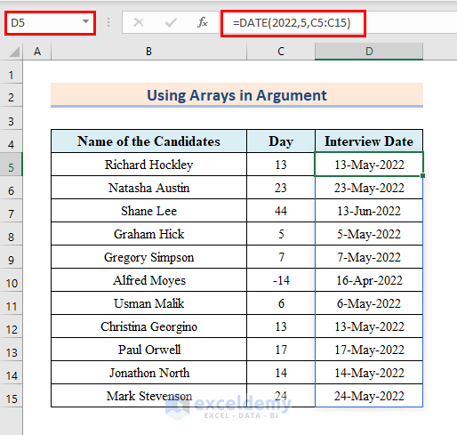
- Enter the following formula in cell D5:
=DATE(2022,5,C5:C15) In the formula, I imputed an array instead of a specific cell, giving an output array of dates.
Example 1 – Finding the First Day of the Month Using the DATE Function
Steps:
- Enter the following formula in cell D5:
=C5-DAY(DATE(2022,9,15))+1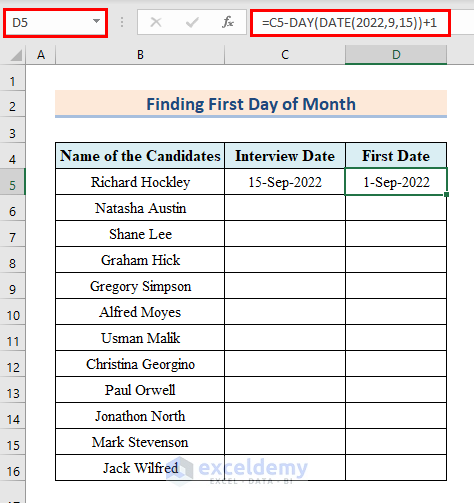
You can find out the dates for other candidates in a similar fashion.
Example 2 – Inserting the Last Day of Month with EOMONTH and DATE Functions
Steps:
- Enter the following formula in cell D5:
=EOMONTH(DATE(2022,2,12),0)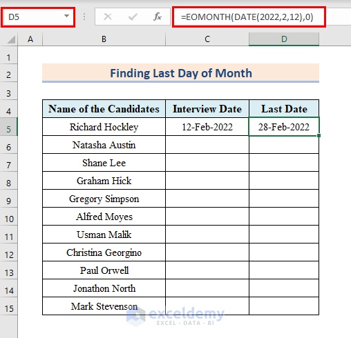
- Press Enter.
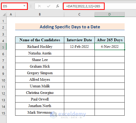
Example 3 – Applying the Excel DATE Function to Add Specific Days to Date
Steps:
- Enter the following formula in cell D5:
=DATE(2022,2,12)+265- Press Enter.
The formula will return the date after adding 265 from the DATE function.
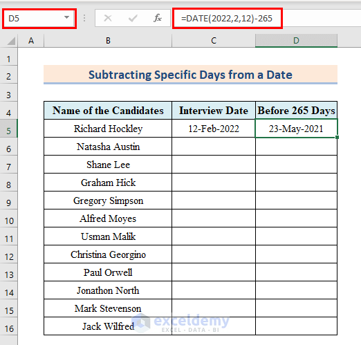
Example 4 – Using the DATE Function to Subtract Specific Days from Date
Steps:
- Enter the following formula in cell D5:
=DATE(2022,2,12)-265- Press Enter.
In the formula, we simply subtracted 265 from the date output of the DATE function.
- The formula returns the date back to 265 days.
- We can subtract any number instead of 265 in the formula.
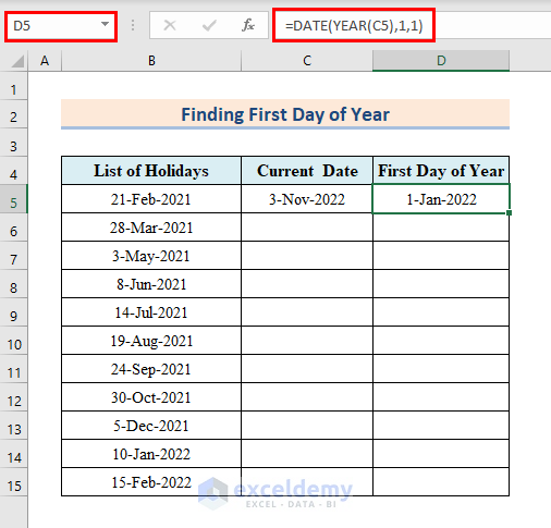
Example 5 – Identifying the First Day of the Year with DATE and YEAR Functions
Steps:
- Enter the following formula in cell D5:
=DATE(YEAR(C5),1,1)- Press Enter.
We will see the 1st date of the year as a result.
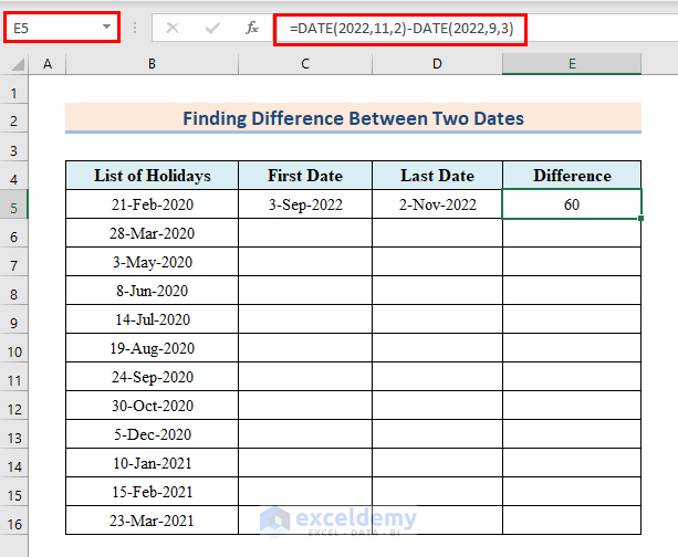
Example 6 – Counting Days Between Two Dates in Excel
Steps:
- Enter the following formula in cell E5:
=DATE(2022,11,2)-DATE(2022,9,3)- Press Enter.
The formula will give the difference between two dates and the output of two DATE functions.
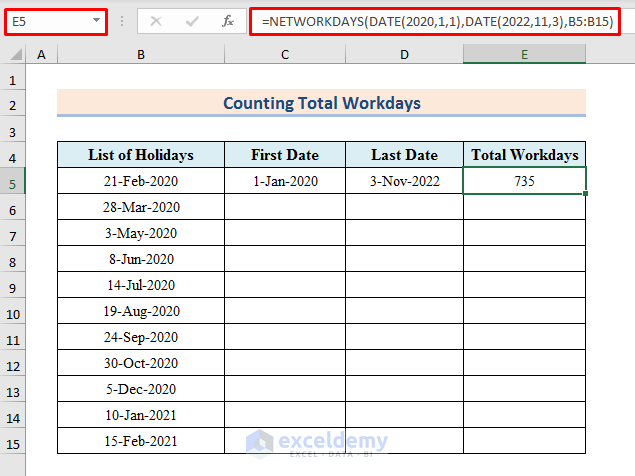
Example 7 – Counting Total Workdays Between Two Dates in Excel
Steps:
The syntax of this function is:
=NETWORKDAYS(start_date,end_date,[holidays])Here, start_date is the starting date, end_date is the ending date and [holidays] is a list of holidays.
To find the workdays between 1-Jan-2020 and 3-Nov-2022,
- Enter the following formula in cell E5:
=NETWORKDAYS(DATE(2020,1,1),DATE(2022,11,3),B5:B15)- Press Enter.
We will see the net workdays between the two dates excluding the holidays also.
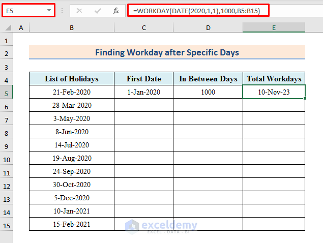
Example 8 – Finding the Workday after a Specific Number of Days in Excel
Steps:
The Syntax of the WORKDAY function is:
=WORKDAY(start_date,days,[holidays])To find the workday after 1000 days starting from 1 January 2020, with B5:B15 as a list of holidays,
- Select cell E5.
- Enter the formula below:
=WORKDAY(DATE(2020,1,1),1000,B5:B15)- Press Enter to see the result.
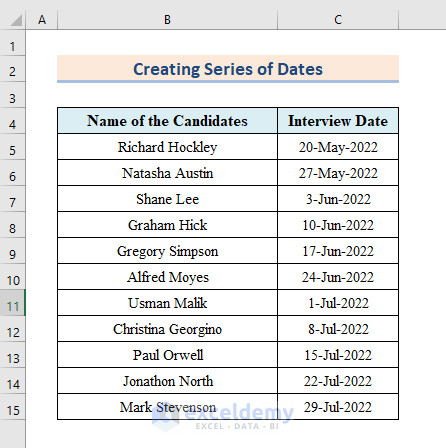
Example 9 – Creating a Series of Dates in Excel
Steps:
- Enter the following formula in cell C5:
=DATE(2022,5,20)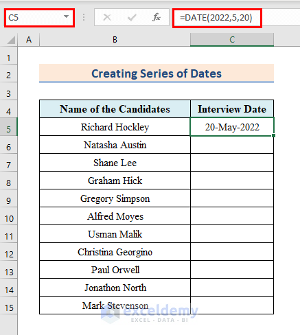
- Press Enter.
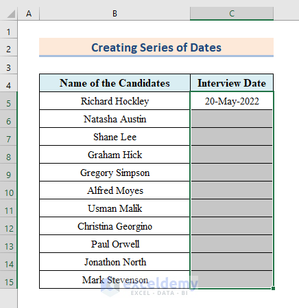
- Select the range of cells C5:C15 to create the arrays.
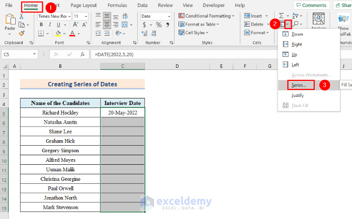
- Go to the Home tab.
- Click on the small icon beside Fill and select Series.
- The Series window will pop up.
- Select Column, Date, and Day in the box.
- In the Step value box write 7. It will create a gap of 7 days in between dates.
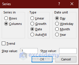
- Press OK, and we will see the series of dates created.
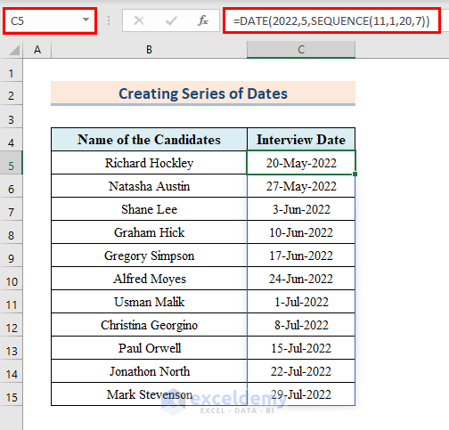
- Instead of using the procedure mentioned above, you can use the following formula to create a series of dates.
=DATE(2022,5,SEQUENCE(11,1,20,7))- Next, hit Enter and we can see the series of dates created.
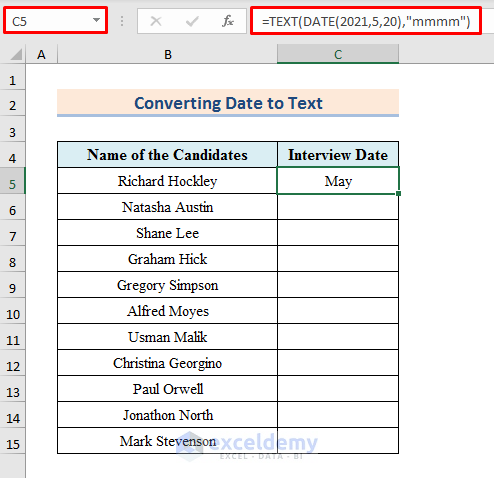
Example 10 – Converting the Date to Text with TEXT and DATE Functions
Steps:
The syntax of the TEXT function is:
=TEXT(value,format_text)Here, value is the value that will be converted to text, and format_text is the format in which you want to get your texts. Excel accepts a lot of text formats.
To extract the text names of the month of any date,
- Select cell C5 and enter the formula below:
=TEXT(DATE(2021,5,20),"mmmm")- Press Enter to see the result.
Common Errors with Excel DATE Function
The VLOOKUP function has the following common errors.
| Error | When They Show |
|---|---|
| #NUM! | Shows when it finds wrong arguments or large numbers. |
| #VALUE! | Shows when the argument number is of the wrong data type, like text, array, etc. |
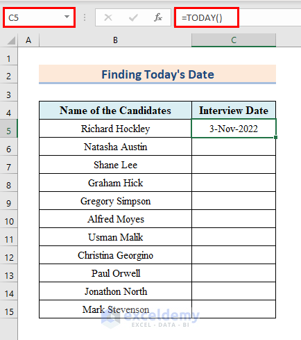
How to Insert TODAY Function to Get Today’s Date in Excel
We can easily find today’s date in Excel using the TODAY function. Let’s follow the procedures given below.
- Enter the following formula in cell C5 and press Enter.
=TODAY()- It will give today’s date as output.
Download the Practice Workbook
You can download the practice workbook.
<< Go Back to Excel Functions | Learn Excel
Get FREE Advanced Excel Exercises with Solutions!
