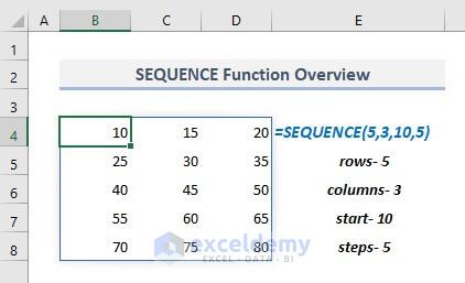
Here’s a brief overview of SEQUENCE(5,3,10,5). To learn exactly how we got there, follow the instructions below.
Introduction to the SEQUENCE Function
- Function Objective:
The SEQUENCE function is used to create a sequence of numeric values.
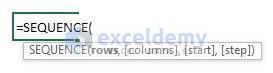
- Syntax:
=SEQUENCE(rows, [columns], [start], [step])
- Arguments Explanation:
| Argument | Required/Optional | Explanation |
|---|---|---|
| rows | Required | The number of rows. |
| [columns] | Optional | The number of columns. |
| [start] | Optional | Start number in the return array. |
| [step] | Optional | The common difference between successive two values in the sequence of numbers. |
- Return Parameter:
An array containing a sequence of numbers with the defined specifications.
How to Use SEQUENCE Function in Excel: 16 Examples
Part 1 – Basic SEQUENCE Function with Only One Argument
The first argument of the SEQUENCE function is ‘rows’ which indicates the number of rows to be shown in the spreadsheet. If you don’t input any other arguments, the function will fill in cells in the specified number of rows where the first cell will contain the number ‘1’ and later all other sequential numbers will be displayed in the following rows.
So, in the picture below, Cell B4 contains the formula:
=SEQUENCE(5)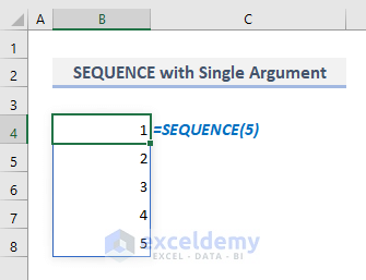
Part 2 – SEQUENCE Function with Two Arguments in Excel
Since the second argument of the function denotes the number of columns, using two arguments will result in an array of the specified rows and columns, sequenced from left to right then top to bottom.
Consider this example where the Cell B4 contains the SEQUENCE function with rows and columns:
=SEQUENCE(5,3)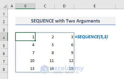
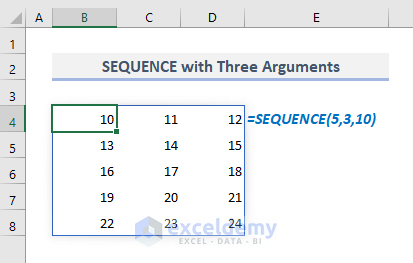
Part 3 – SEQUENCE Function with Three Arguments in Excel
Now the third argument of the function is [start], which denotes the starting value or number to be shown in the first cell of the first row in an array.
Consider the following formula in Cell B4. With the first three arguments, the function will return the array as shown in the following screenshot.
=SEQUENCE(5,3,10)Where the starting value is 10 in the array that has been defined in the third argument of the function.
Part 4 – SEQUENCE Function with Four Arguments in Excel
The fourth argument of the function, [step], denotes the interval between any two successive values in the array.
Suppose we want to build an arithmetic series of integer numbers starting from 10 where the step is 5.
The required formula in Cell B4 will be:
=SEQUENCE(5,3,10,5)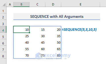
Part 5 – Use of SEQUENCE Function to Generate Dates or Months in Excel
Method 1 – Creating Sequential Dates with SEQUENCE and TODAY Functions
Suppose we want to create a list of ten successive dates starting from the current date. The related formula in Cell B5 should be:
=SEQUENCE(10,1,TODAY(),1)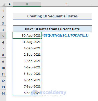
Method 2 – Creating a List of First Dates for Sequential Months with EDATE and SEQUENCE Functions
Let’s say we want to show the first dates of all months in the year 2021. So, in the output Cell B4 in the following picture, the required formula will be:
=EDATE(DATE(2021,1,1),SEQUENCE(12,1,0))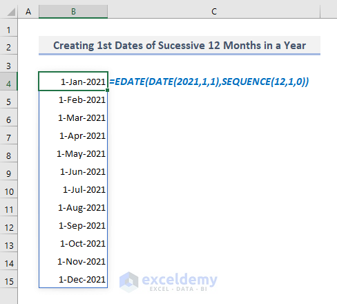
Method 3 – Making a List of 12-Month Names with SEQUENCE Function in Excel
The required formula in Cell B5 should be:
=TEXT(EDATE(DATE(2022,1,1),SEQUENCE(12,1,0)),"mmmm")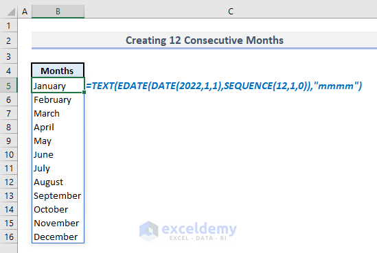
Part 6 – Combination of SEQUENCE and TRANSPOSE Functions in Excel
By applying the SEQUENCE function with all four arguments inside, we can create an array of some sequential numbers and the flow of the numbers will be from left to right, like in the picture below.
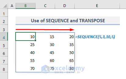
Suppose we want to display the sequence of these numbers from top to bottom in the array. The required formula in the output Cell B10 should be:
=TRANSPOSE(SEQUENCE(5,3,10,5))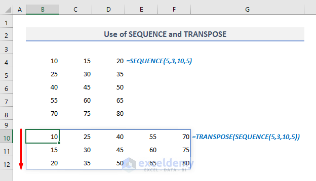
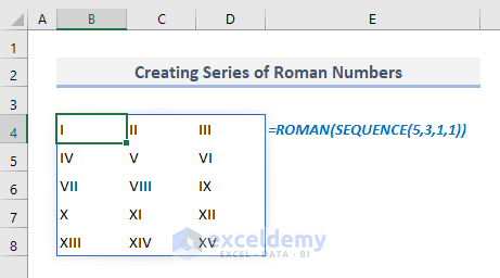
Part 7 – Creating a Sequence of Roman Numbers in Excel
The required formula in any cell should be:
=ROMAN(SEQUENCE(5,3,1,1))This will create the fifteen successive Roman numbers starting from ‘i’ in the array of five rows and three columns.
Part 8 – Use of SEQUENCE with INDEX Function in Excel
Let’s have a look at the dataset below. Each smartphone brand and its model appear twice in the table: one is with the actual price and another is with a discounted price. Here’s how you can show the rows of all brands containing discounted prices only.
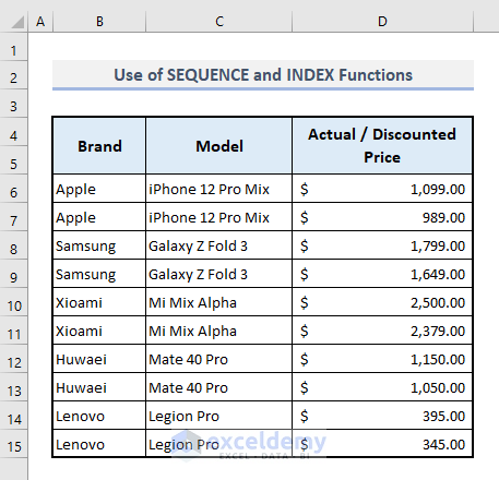
- In the output Cell B18, the related formula will be:
=INDEX(B6:D15,SEQUENCE(COUNTA(B6:B15)/2,1,2,2),SEQUENCE(1,3))- Press Enter, and you’ll get the resulting array with all smartphone brands and model names with their discounted prices only.
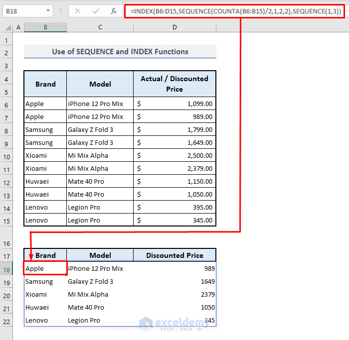
How Does the Formula Work?
➯ COUNTA function counts the total number of cells in the range of B6:B15. Then the output (10) is divided by 2 and the resultant value is inputted as the first argument (rows) of the SEQUENCE function.
➯ In the second argument (row_num) of the INDEX function, the SEQUENCE function defines which rows have to be extracted from the table.
➯ For the third argument of the INDEX function, another SEQUENCE function defines all the columns that have to be considered for extracting data.
Part 9 – Creating a Random Order for SEQUENCE Outputs
For this, we have to use the SORTBY function outside the SEQUENCE function and the sorting will be performed based on the RANDARRAY function where RANDARRAY function returns random numbers with no particular order or sequence.
In Cell B4, the related formula to create a random order for sequential numbers should be:
=SORTBY(SEQUENCE(10),RANDARRAY(10))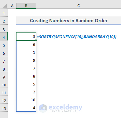
Part 10 – Creating a Dynamic Calendar with SEQUENCE Function in Excel
Assume we have a random date value in Cell C4 and that is 01-08-2021 or 1 August 2021. By incorporating the WEEKDAY function, we can extract the month from that specified date and thereby show all the calendar days for that particular month.
The required formula to display a calendar month based on a date in Cell B7 will be:
=SEQUENCE(6,7,C4-WEEKDAY(C4)+1)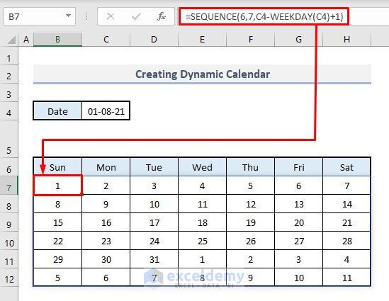
How Does the Formula Work?
➯ In the SEQUENCE function, the number of rows has been defined by 6 and the number of columns by 7.
➯ The start date has been defined by “C4-WEEKDAY(C4)+1”. Here the WEEKDAY function extracts the serial number of the weekday (By default, 1 for Sunday and thus successively 7 for Saturday). The date in Cell C4 subtracts the number of weekdays and later by adding ‘1’, the start date becomes the first date of the prospective month.
➯ The SEQUENCE function then shows the successive dates from left to right in an array of 6 rows and 7 columns. Don’t forget to customize the format of the dates to show only the serial of the days.
Part 11 – Making a Repeated Sequence with the Help of MOD and SEQUENCE Functions
In the following screenshot, integer values from 1 to 4 have been displayed multiple times in a column.
The required formula in Cell B4 to create this array is:
=MOD(SEQUENCE(12)-1,4)+1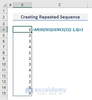
How Does the Formula Work?
➯ Since here the integer values from 1 to 4 are to be shown multiple times, the multiple of 4 has to be assigned as the number of rows in the SEQUENCE function.
➯ “SEQUENCE(12)-1”, this part of the formula returns the following array:
{0;1;2;3;4;5;6;7;8;9;10;11}
➯ MOD function divides each of the integer values in the array with 4 and returns all the remainders in a final array.
Part 12 – Creating Repeated Numbers in a Sequence in Excel
In the picture below, integer values from 1 to 5 have been repeated twice in Column B.
The required formula that has been used to create the return array is:
=ROUNDUP(SEQUENCE(10, 1, 1/2, 1/2), 0)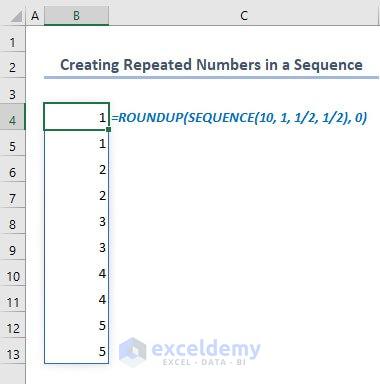
How Does the Formula Work?
➯ Here the start point and the step value in the SEQUENCE function have been assigned with ½ in both cases.
➯ With the mentioned arguments, the SEQUENCE function would return the following array:
{0.5;1;1.5;2;2.5;3;3.5;4;4.5;5}
➯ Finally, the ROUNDUP function rounds up all the decimals to the next integer digit.
Part 13 – Generating Empty Values in a Sequence of Numbers
If you need to leave an empty cell or a space after each value in a sequence of numbers, then you can merge IF, INT, and SEQUENCE functions as well to get the output. In the following picture, the numbers from 1 to 5 have been shown in a sequence with a space after each value in the sequence.
The required formula in Cell B4 is:
=IF(INT(SEQUENCE(10, 1, 1, 1/2))=SEQUENCE(10, 1, 1, 1/2), SEQUENCE(10, 1, 1, 1/2), "")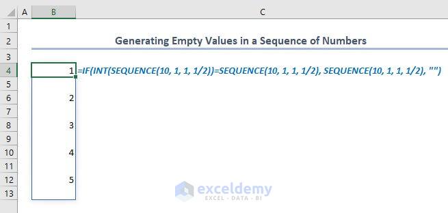
How Does the Formula Work?
➯ SEQUENCE(10,1,1,½), this repeated part of the formula returns the following array:
{1;1.5;2;2.5;3;3.5;4;4.5;5;5.5}
➯ INT(SEQUENCE(10,1,1,½)) returns another array of:
{1;1;2;2;3;3;4;4;5;5}
➯ With the IF function, the formula checks if the values in the second array match with the values in the first one. If the values are matched, the matched rows return with perspective values. Otherwise, the rows remain empty which are considered blank cells in the output column.
Part 14 – Formatting a Sequence of Numbers with Leading Zeros in Excel
Let’s format the output to contain leading zeroes for four digits. The required formula in Cell B4 will be:
=TEXT(SEQUENCE(10,1,5,50),"0000")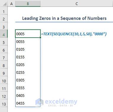
Part 15 – Creating a Reverse Order in a List with SEQUENCE Function
In Column B, there are some random names and in Column D, we’ll display these names in reverse order. So, the required formula in Cell D5 should be:
=INDEX(B5:B10, SEQUENCE(ROWS(B5:B10), , ROWS(B5:B10), -1))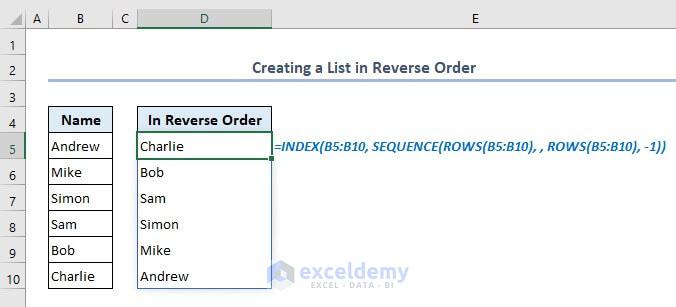
Here, the SEQUENCE function reverses the row numbers of all names and the INDEX function later extracts the names in a reverse order based on the second argument (row_num) modified by the SEQUENCE function previously.
Part 16 – Preparing an Alphabet List with SEQUENCE and CHAR Functions
In the following picture, two separate rows have been used to display the array containing all letters.
The required formula in Cell B4 is:
=CHAR(SEQUENCE(2,13,65))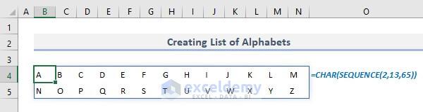
In this formula, the CHAR function returns the characters specified by the Unicode. As there are 26 letters in English, we have used 13 columns here. We can also define the column number as 2 and the formula will return all the letters in 13 rows and 2 columns.
Things to Keep in Mind
SEQUENCE function returns an array by spilling the values in multiple rows and columns. So, if any of the return values in the array cannot find an empty cell to represent itself then the function will return an #SPILL error.
SEQUENCE function is currently available in Microsoft Office 365 only.
The default value for all optional arguments of the SEQUENCE function is 1.
Download Practice Workbook
You can download the Excel workbook that we have used to prepare this article.
<< Go Back to Excel Functions | Learn Excel
Get FREE Advanced Excel Exercises with Solutions!

Didn’t ever notice that using TRANSPOSE on SEQUENCE would be different than reversing row/column values in it ( SEQUENCE(5,3) vs. SEQUENCE(3,5) ). But the reversing goes across columns, then down a row, and repeats while with TRANSPOSE, it goes down a column, over one column, down, and repeats.
I liked especially the generating blanks one. I’m sure there’re lots of ways to do this, but this seems like an easy way to select every n-th item in a column.
The one that gives my heart joy though, since I can use it as a simple, simple, simple way to generate card lists and dice rolls in games, is the random ordering one.
Thanks!
Honorable mention to the {1,2,3,4,1,2,3,4,etc.} one. I know I’ll find a use for that.
Thank You, Roy, for your precious comment!
By the way, the sequence, #9 above, that I will happily use for card lists and dice rolls (and I’m sure other things as well)… of course, due to the RANDARRY function, they are volatile and change upon recalc. Since recalc is hard to avoid when one desires to recalc(!), how does one keep the list as long as it should be kept without somehow converting it to values, then later recovering the formula to use again, all the while not having to do it by hand so as to keep gameplay as gameplay rather than an exercise in mousing about and pasting special and so on? Formulaicly would be nice as one might want to minimize use of VBA, or not use it at all if possible.
Turns out, an old Excel 4 Macro command comes to the rescue.
Excel has recently actually begun truly wiping them out as they gave folks, especially organizations, the ability to exclude them via the Trust Center, but also because, while they would warn you to save as macro spreadsheets (.xlsm, say), you could actually ignore that and save as an .xlsx yet still have everything still there when re-opening the spreadsheet. Not now. If not saved as a macro spreadsheet, they are wiped upon saving.
So, maybe not available for too much longer as these things, and others I may not be aware of, of course, are direct attacks on people using them with the obvious intent of, one day soon (sooner, not later), eliminating their existence.
It’s been 25-30 years without much more than neglect, but I wager that within two new versions, they will be utterly gone.
In any case, they exist now. And if one sets the formula (#9’s in this case) in a Named Range, then uses a second Named Range to EVALUATE it, then the result of that second Named Range is NOT ONLY non-volatile, but it works with SPILL array functionality so all the elements of the array are present for other formulas to use or to display in a list as you’d expect, if you wish to do that.
So using that trick, which I wager would be good for other volatile functions since SEQUENCE is a modern, cell-side function itself, one gets a stable array even though one of the elements of the array’s formula, RANDARRAY, is itself volatile.
Not related, but something else representing a still useful difference in functionality, is that some Excel 4 Macro commands have modern, cell-side functions that replace them. However, the new functions often have limitations in respect to the earlier functions and those differences can make a… difference.
Using CELL(“width”) gets you an integer value for the cell width whatever its true width is. GET.CELL(16,A1) shows the measurement you’d see examining it’s properties, so if 8.63, then 8.63, not 8. Minor, but normally what you actually want.
Modern, cell-side FORMULATEXT returns the formula in a cell, including “=” sign, IF ANY FORMULA IS PRESENT, as text for use. If any formula is present, and errors otherwise. But GET.CELL(6,A1) or GET.CELL(41,A1) return whatever is in the cell, so if the constant value 8 is there, “8” is returned, not an error. A nice way to avoid error handling, if nothing else.
Not to mention that since I now have to save as a macro file anyway, there’s no inhibition to using the old macro sheets (Ctrl-F11 to insert one). VBA is much mor ecapable, no question, but harder to use. Macro sheets from “back in the day” are pretty simple to write with new functions easy to find and understand while VBA references… not so much, really. And seconday considerations are often needed with VBA as well. Specify a range? Oh, just type A1:A4. Oh. No? Not even close? Range(A1:A4)? Good… Oh… no? Range(“A1:A4”)? Good… Oh… no? Ah, .Range(“A1:A4”). Yay! I think… yes, seems that works… secondary knowledge is needed for almost every function or command. Not so with Excel 4 Macros.
But… oh no… they are really going away… THAT’s an inhibition. (Sigh…)
Still, while they still work… For the differences!
Especially until they give us a cell-side EVALUATE, and the glorified LET they call LAMBDA does NOT look like that will do, I hope they keep the Excel 4 Macro commands working. EVALUATE is soooo much more than INDIRECT. There’s really little comparison.
Lordy, LAMBDA. Been making Named Range functions, as in they can take parameters, for 25 years now. LAMBDA will make that easier (literally a million times easier, very little exaggeration here, and why I have not made thousands in that time, rather a couple dozen only) and better, sure, NO question at all, but it isn’t new capability! And not much differnt than LET already is. Marketing… (shudder).
Hello Roy! Thank you for your comment. I must say your knowledge of Microsoft Excel is really appreciable. Keep commenting on posts of Exceldemy and help others to learn more.
Is it possible to make in sequence formula in excel 100A, 101B, 102C, 103D, 104A, 105B, 106C, 107D so on and on. Thanks
Hello Johan, you can use the following procedure to serve your purpose-
– Make a column with 101, 102, 103, and so on.
– Make a column with A, B, C, D, and repeat.
Follow this article to repeat numbers or characters serially.
How to Add Numbers 1 2 3 in Excel
– Then use CONCATENATE function to combine them.
Let us know the outcome in the reply. Thank you!
Trying to create a sequence formula to insert a date(s) to begin at 1st day of month corresponding to day of week in a column. I have a worksheet with (12) different sequence formulas, one for each month, based on a given “input” year. Would like to only populate actual dates in each month. Right now am populating all (37) possible day options in columns.
I can send you a screenshot or copy of present file. Thanks for any suggestions.
2-19-2023
Good day, Don Rogers.
Thank you for your feedback. Could you please share your excel file with me so that I can better understand your problem and provide you with a solution? You can shareyour file to the email address provided below.
[email protected]
Thank you!
Here is another example that will fill a list with the same value is growing dynamically with the list size.
=SWITCH(SEQUENCE(COUNTA(a_list)-1),1,”Word_to_repeat”,”Word_to_repeat”)
Hey Yann, we have tried your formula. But unfortunately, this formula is not working as you said it would. It gives a Value error instead.
Hi, how can I extend the INDEX & SEQUENCE function with a COUNTIF that there then (0/1/2/etc.):Text-of-LIST!B2:B30
[1:volcano]
[1:village]
[1:city]
[2:village]
comes out
=INDEX(List!$B$2:$B$30;SEQUENCE(ANZAHL2(List!$B$2:$B$30)/1;1;1;1);SEQUENCE(1;1))
=COUNTIF(List!$B$2:B2;List!B2)&”:”&List!B2
Hello DOMJI,
I cannot understand why are you trying to combine these two formulas. You can get your desired output just by using the formula with the COUNTIF function.
=COUNTIF($B$2:B2,B2)&":"&B2Using this formula, you can get the [Occurrence: Item] format in the output. You cannot use the COUNTIF function with INDEX and SEQUENCE functions as they return array output.
Hope this helps. Let us know if you have any other things to know.
Regards,
SHAHRIAR ABRAR RAFID
Team ExcelDemy