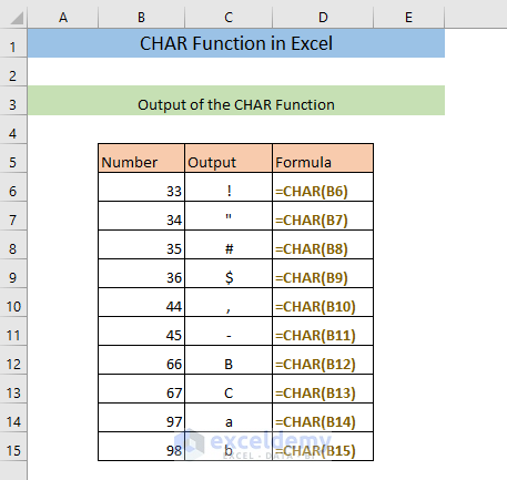
How to Use the CHAR Function in Excel

The American System Code for Information Interchange, or ASCII, is a character encoding standard used in digital communications. A unique integer number is assigned to each character that can be entered in the CHAR function. The character can be a number, alphabet, punctuation marks, special characters, or control characters. For Example, the ASCII code for [comma], is 044. The lowercase alphabets a-z have ASCII values ranging from 097 to 122.

The CHAR Function

Objective

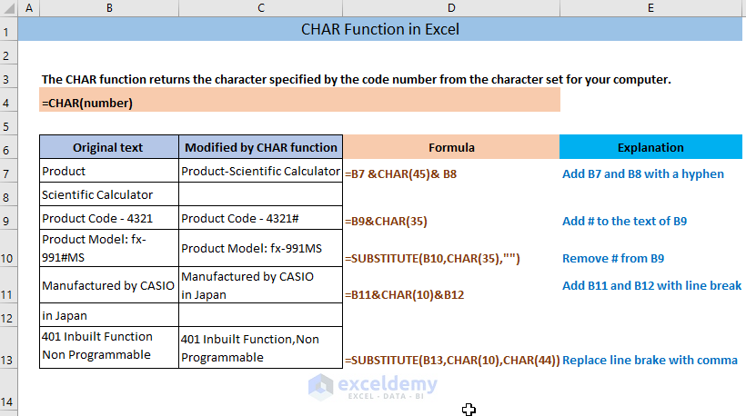
The CHAR function returns the character specified by its code number.

Syntax

CHAR(number)

Argument Explanation

Argument	Required/Optional	Explanation
number	Required	A number between 1 to 255 assigned to a specific character

Output

The CHAR function returns a character based on the number given as argument.

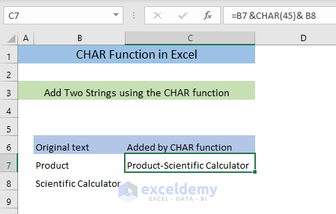
Example 1 – Add Two Strings Using The CHAR Function

Enter the following formula in an empty cell (C7),

=B7 &CHAR(45)& B8

The formula will add the strings in B7 and B8 with a hyphen and return the output in C7. (to add other characters, insert a different code. For example, 44 for comma or 32 for a space).

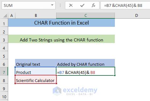
Press ENTER.

You’ll see the two strings joined by a hyphen in C7.

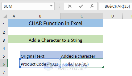
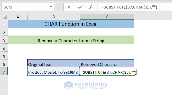
Example 2 – Add a Character to a String

To add a # to the product code:

Enter the following formula in an empty cell (C7).

=B6&CHAR(35)

The formula will add a # (code 35) to the text in B6 and return the output in C7.

Press ENTER.

You’ll see a # added to the text in C7.

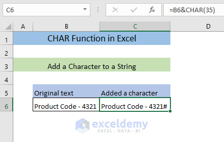
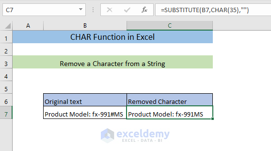
Example 3 – Remove a Character from a String

To remove the # from the string in B7:

Enter the following formula in C7.

=SUBSTITUTE(B7,CHAR(35),"")

The CHAR function will return the character # for the code 35 and the SUBSTITUTE function will remove it from B7, replacing it with an empty string.

Press ENTER.

The character was removed.

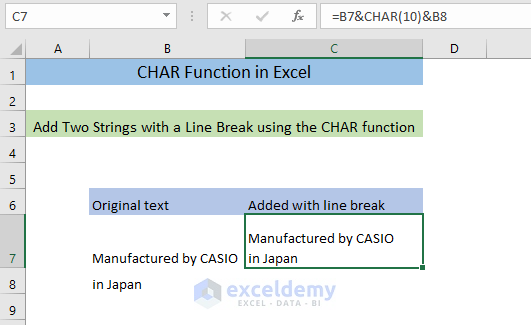
Example 4 – Add Two Strings with a Line Break Using the CHAR Function

Enter the following formula in C7.

=B7&CHAR(10)&B8

The formula will join the texts in B7 and B8 with a line break (character code 10).

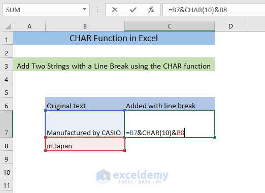
Press ENTER.

This is the output.

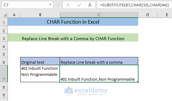
Example 5 – Replace a Line Break with a Comma using the CHAR Function

Enter the following formula in C7.

=SUBSTITUTE(B7,CHAR(10),CHAR(44))

CHAR(10) returns a line break and CHAR(44) returns a comma. The SUBSTITUTE function replaces the line break with a comma.

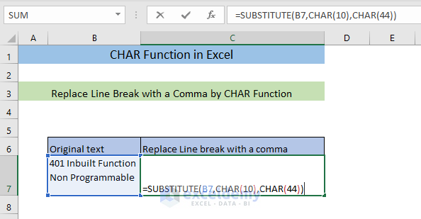
Press ENTER.

This is the output.

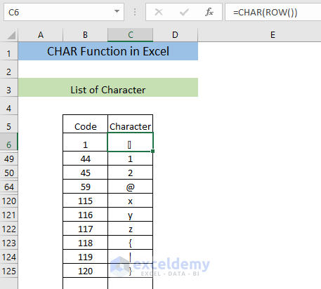
Example 6 – Using the CHAR Function to Create a List of Characters

Enter the following formula.

=CHAR(ROW())

The formula returns the first character.

Press ENTER.
Drag Fill Handle to the 255th cell.

You will get the complete list of the characters.

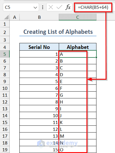
Example 7 – Create a List of Alphabets in Excel

Create a list of numbers from 1 to 26 for each alphabet letter.
Use the following formula.

=CHAR(B5+64)

64 was added to each serial number as the alphabet code starts from 65.

Example 8 – Check If the ASCII Values Are Correct for a List of Characters

Use the function:

=IF(CHAR(C5)=B5,"Correct","Incorrect")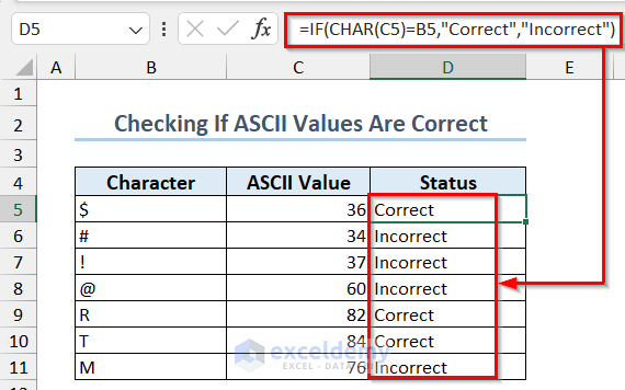

Read More: How to Convert Excel ASCII to Char

Things to Remember When Using The CHAR Function

The CODE function can be used as a reverse CHAR function. For example, enter =CODE(“A”), it will return 65.
The CHAR function can not return all characters. For advanced characters, use the UNICHAR function.