Character Codes for CHAR Function in Excel (5 Common Uses)

Looking for a way to use Excel character codes for the CHAR function? Don’t worry, you have come to the right place. In this article, I will show you how to use character codes for the CHAR function in Excel.

Excel Character Codes

There are different types of characters used in Excel like letters (a, b, c), numbers (0, 1, 2, 3), punctuations ( , . :), and some special characters (@, #, ! ), etc. A user can type most of the characters with the help of a keyboard. But we can’t enter the special characters using the keyboard. However, for each character, a code is defined in the system of the computer. ASCII (American Standard Code for Information Interchange) represents code for computers, telecommunication equipment, and some other devices.

Excel CHAR Function

The CHAR function in Excel returns a special character when any valid number is applied to this function. According to ASCII, any number between 1 to 255 has a distinctive character assigned to it on a computer. So, the argument of the CHAR function is the code of the corresponding character. For example, the code for a hyphen is 45. So, CHAR(45) will return a hyphen.

Character Codes with Excel CHAR Function

Let’s say, we have some character codes in an Excel worksheet. The names of the characters and corresponding CHAR functions are available here.

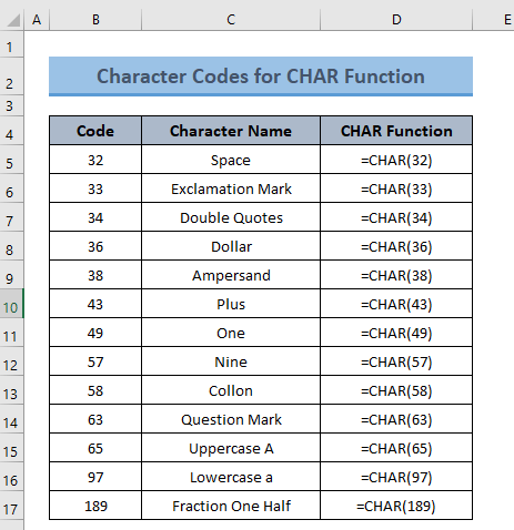
We have shown the formulas instead of showing the values. Now we want to show the symbols using the CHAR function. In order to do so, proceed with the following steps.

• Select a cell (i.e. E5) where you want to show the symbol and type the following formula in the selected cell.

Here,
B5 = Character code

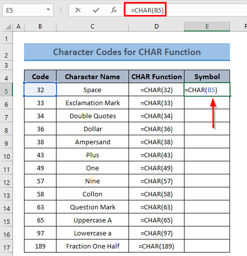
• Press ENTER and you will see the cell blank as the code for the character space is 32.
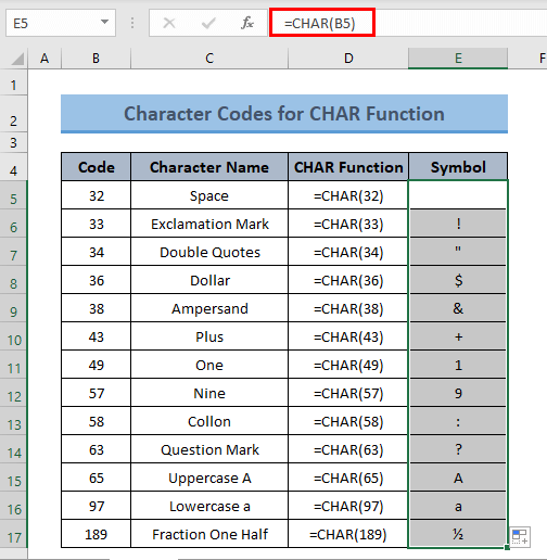
• Now, use the Fill Handle tool to Autofill the formula down to the cells.

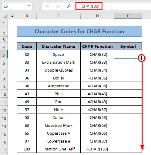
• Hence, all the formulated cells will show the specific character for the corresponding code.

In this section, I will discuss adding, removing, and replacing some characters by using codes with the help of the CHAR function.

1. Adding Two Strings with “Space”

Sometimes you may need to add two text strings together in your worksheet. When you need to do these types of corrections for a number of cells, it’s okay to do it manually. However, it is not a wise approach for a large number of cells and dynamic sheets. Here, applying the character codes using the CHAR function will definitely make your task easy and dynamic.

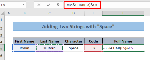
Let’s say, we have the first name and last name of a person and we want to add these two texts with a space between them. The character code for space is 32. Let’s see how you can connect these two text strings.

• Firstly, select a cell where you want to add the text and type the following formula in it.

Here,

B5 = First text
C5 = Last yext
E5 = Character code of space

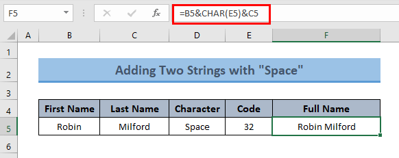
• Now, press ENTER and you will see that the two texts have been connected with a space between them.

Read More: How to Use Code 9 with Excel CHAR Function

2. Adding Hyphen to a Text

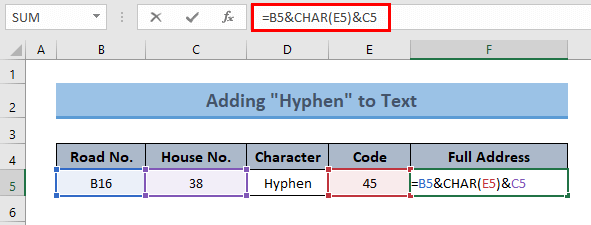
A user can add two texts with hyphens by using the character code nested in the CHAR function. In our data, we have the Road No. and House No. of a person and we want to show the full address by connecting these two texts with a hyphen. In order to do so, just proceed with the steps below.

• First of all, select a cell and type the following formula in the cell.

Here,

B5 = First text
C5 = Last text
E5 = Character code of hyphen

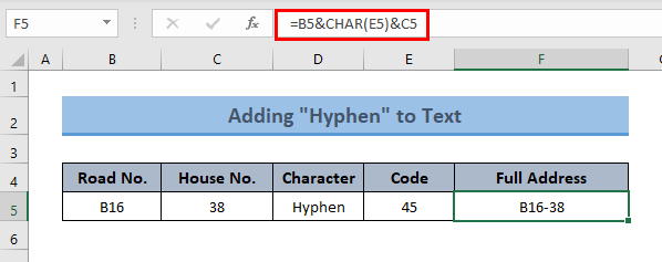
• Then, press ENTER, and it will add the two texts connected with a hyphen (i.e. B16-38).

Read More: How to Use CHAR(10) Function in Excel

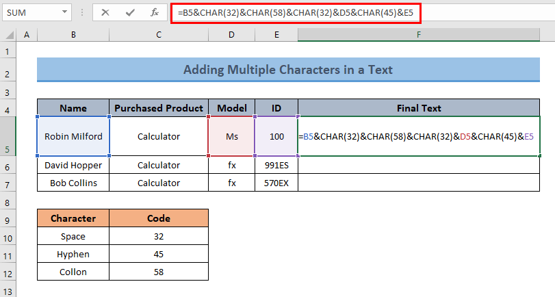
3. Adding Multiple Characters in a Text

You can not only add single characters using the CHAR function but also add multiple characters between texts with character codes. In the example below, I have added space, hyphen, and colon between texts.

• Select a cell to show the output and type the following formula in it.

Here,

B5 = First text
D5 = Middle text
E5 = Last text
32 = Character code of space
45 = Character code of hyphen
58 = Character code of collon

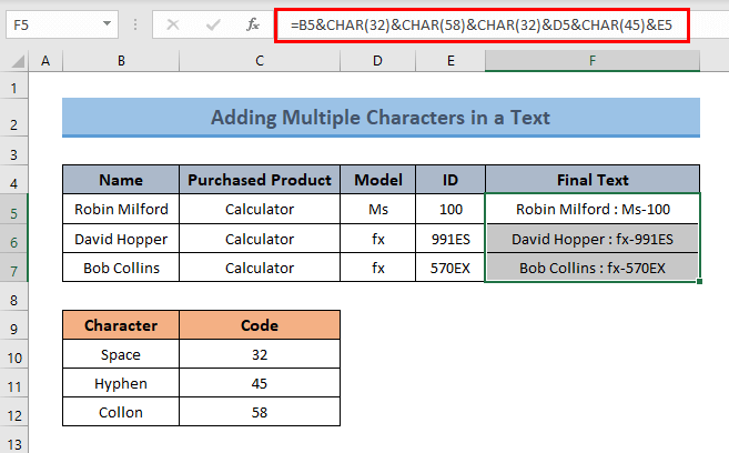
• Press ENTER, and the cell will show the text by adding these three characters. You can add as many characters as you want.

Read More: How to Use CHAR(32) Formula in Excel

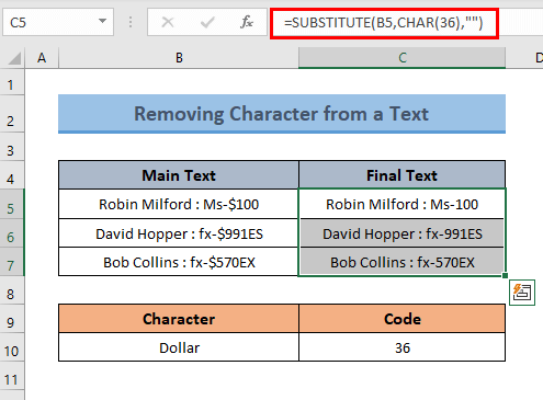
4. Removing Character from a Text

Excel also allows a user to remove characters using the codes. For this, we have to use the CHAR function nested with the SUBSTITUTE function. The SUBSTITUTE function substitutes the referred characters, texts, or cells.

Here, our dataset includes a Dollar ($) sign and we want to remove this character. The character code for the Dollar is 36. Just apply the following formula in the cell.

Here,
B5 = First text
36 = Character code of dollar

The SUBSTITUTE function removes the character with code 36 and puts a blank space.

Read More: How to Use CHAR(34) Formula in Excel

5. Replacing Character in a Text

If you want to replace the Dollar ($) sign with a Hash (#), then apply the following formula.

Here,

B5 = First text
36 = Character code of dollar
35 = Character code of hash

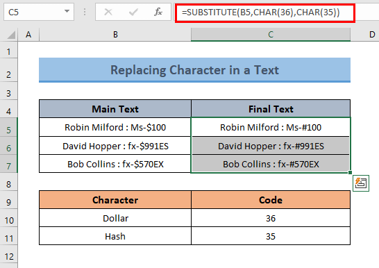
The SUBSTITUTE function removes the character with code 36 and replaces it with a character whose code is 35. So, $ is replaced by #.

Read More: How to Convert Excel ASCII to Char

Download Practice Workbook

You can download the practice book from the link below.

Conclusion

In this article, I have tried to show you some uses of character codes for the CHAR function in Excel. Hope the article helped you. If you have better methods, questions, or feedback regarding this article, please don’t forget to share them in the comment box. For more queries, kindly visit our website. Have a great day!

Related Articles

• How to Insert a New Line Using CHAR Function in Excel
• [Fixed!] CHAR(10) Is Not Working in Excel