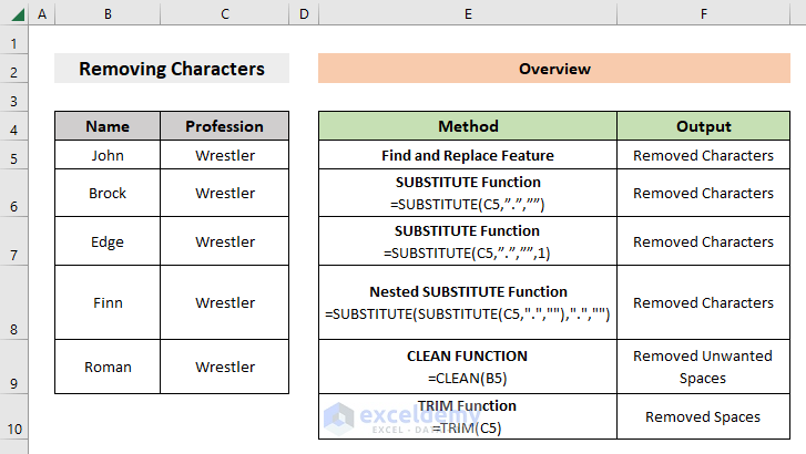
Here’s an overview of removing characters with various functions.
Download the Practice Workbook
6 Methods to Remove Characters in Excel
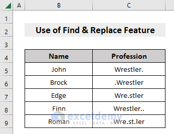
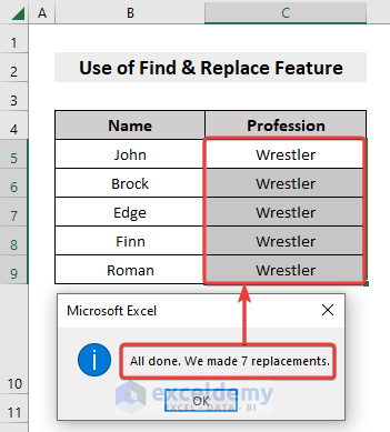
Method 1 – Remove Specific Characters with the Find and Replace Feature
Below is the dataset consisting of Name and their Profession, where the Profession contains unnecessary dots (.), which we’ll remove.
Steps:
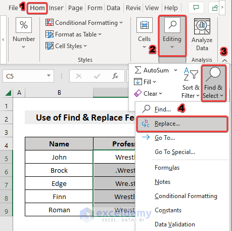
- Select the dataset.
- Under the Home tab, go to Find & Select and choose Replace.
- From the pop-up Find and Replace box, in the Find what field, write the dot (.)
- Leave the Replace with field blank.
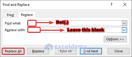
- Press Replace All.
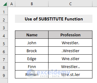
Method 2 – Delete Specific Characters with the SUBSTITUTE Function
The SUBSTITUTE Formula,
=SUBSTITUTE(cell, “old_text”, “new_text”)new_text = the text that you want to replace with
We’ll use the same dataset to remove extra periods.
Steps:
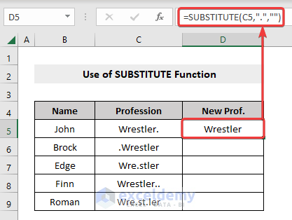
- In an empty cell where you want your result to appear, put an equal (=) sign and then write SUBSTITUTE along with it.
- Inside the brackets of the SUBSTITUTE function, write the cell reference number from which you want to remove dot (.) (in our case, the Cell number was C5).
- Put a comma (,) symbol and write a dot (.) inside double quotes (or any old text that you want to remove).
- Put a comma (,) and leave a blank double quote if you want a null string instead of a dot (.) (or any new string that you want your old text to replace with).
The required formula will look like the following,
=SUBSTITUTE(C5,”.”,””)- Press Enter.
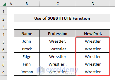
- Drag the row down using the Fill Handle to apply the formula to the rest of the dataset.
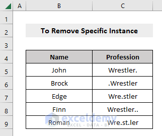
Method 3 – Extract Only a Particular Instance of a Specific Character in a String
Instead of removing all the dots (.) from the Wrestlers’ Profession of the dataset, we will delete only the first dot (.) from each cell.
Steps:
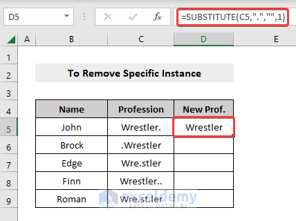
- Use the following formula:
=SUBSTITUTE(C5,”.”,””,1)Here, 1 as the fourth argument means we want to remove the 1st dot (.) from the dataset (if you want to remove the 2nd character from your dataset, write 2 instead of 1, and so on).
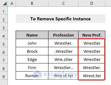
- Drag the row down using the Fill Handle to apply the formula to the rest of the dataset.
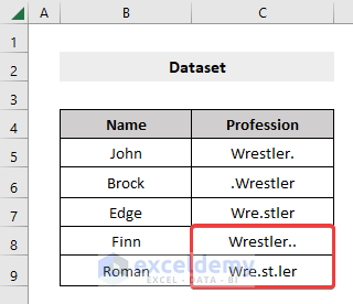
Method 4 – Remove Multiple Specific Characters with a Nested SUBSTITUTE Function
In the dataset below, the Professions for the names Finn and Roman consist of multiple dots (.).
Steps:
- To establish a nested SUBSTITUTE function, you have to write a SUBSTITUTE function inside another SUBSTITUTE function and pass relevant arguments inside the brackets.
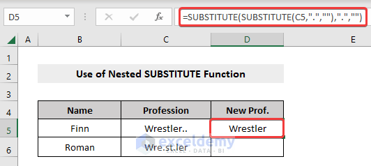
- We start with the formula,
=SUBSTITUTE(C5,”.”,””)- To delete another dot(.) (or any other character that you required) along with it, we put this formula inside another SUBSTITUTE formula and pass the arguments (old_text, new_text) inside it (in our case, it was “.”,””).
- The new formula is:
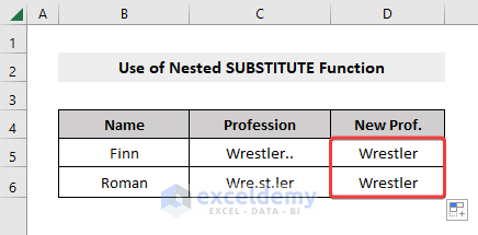
=SUBSTITUTE(SUBSTITUTE(C5,".",""),".","")- Press Enter.
- Drag the row down using the Fill Handle to apply the formula to the rest of the dataset.
Read more: How to Remove Special Characters in Excel
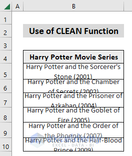
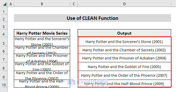
Method 5 – Erase Any Special Characters with the CLEAN Function
The CLEAN function removes line breaks and non-printable characters from a string:
=CLEAN(original_string)original_string = the text or reference to the text cell that you want to clean.
In the following data table, we copy and pasted the Harry Potter Movie Series in the Excel sheet. The cells contain multiple non-printable characters (line-breaks).
Steps:
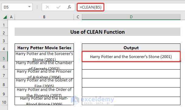
- Select the first cell of the column where you want the results to appear (in our example, it is Cell D5).
- Use the formula:
=CLEAN(B5)
- Press Enter.
- Drag down the Fill Handle to apply the formula to the rest of the dataset.
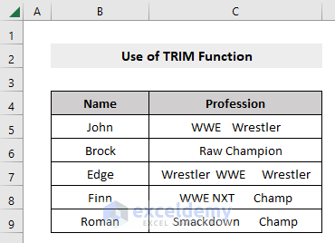
Method 6 – Eliminate Spaces with the TRIM Function
The TRIM function removes all the leading or trailing spaces in texts and extra spaces between words, leaving just a single space.
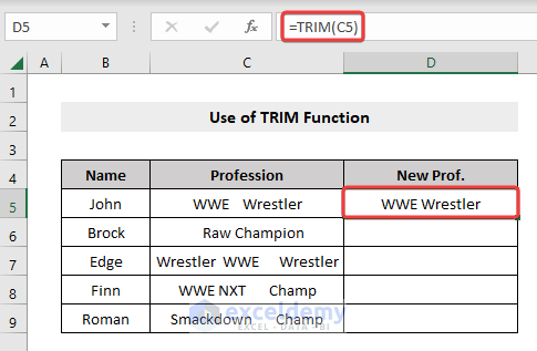
The general syntax for this function is:
=TRIM(original_string)original_string = the text or reference to the text cell that you want to process.
Consider the following dataset where cells contain multiple spaces.
Steps:
- Select the first cell of the column where you want the results to appear (in our example, it is Cell D5).
- Insert the formula:
=TRIM(C5)
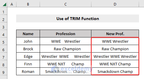
- Press Enter.
- Drag down the Fill Handle to apply the formula to the rest of the dataset.
Keep in Mind
There are many non-printable characters in Unicode that CLEAN cannot remove. The CLEAN function only removes the first 32 (non-printable) characters in the 7-bit ASCII code (i.e., values 0 to 31). Apply the TRIM function after applying the CLEAN function to remove the spaces since the space character has a value of 32 and the CLEAN function won’t remove them.
Excel Remove Characters: Knowledge Hub
- Remove Non-numeric Characters from Cells in Excel
- Remove Non-Alphanumeric Characters in Excel
- Remove Characters from String Using VBA in Excel
- Remove Characters After a Specific Character in Excel
- Excel Remove Characters From Right
<< Go Back To Excel Remove Characters | Data Cleaning in Excel | Learn Excel
Get FREE Advanced Excel Exercises with Solutions!
