How to Remove Special Characters in Excel

This article describes various ways to remove special characters in Excel.

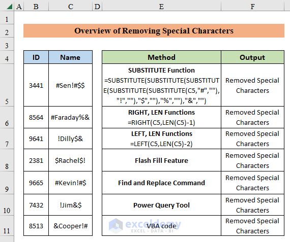
Here’s an overview of the methods and formulas we’ll be applying.

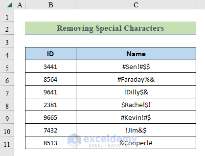
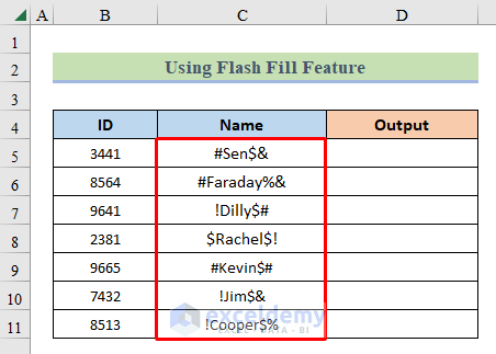
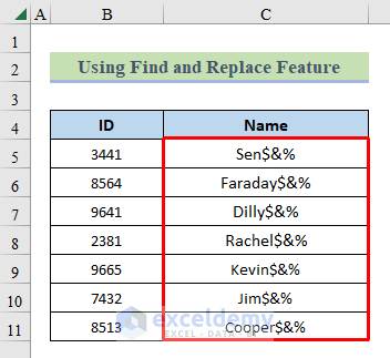
Suppose we have a dataset containing the ID and Name of some Employees. The names contain some special characters. Let’s remove them!

Method 1 – Using Excel Functions

We can construct a formula using functions like SUBSTITUTE, RIGHT, and LEFT to remove special characters.

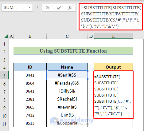
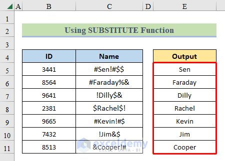
1.1  – Using the SUBSTITUTE Function

The SUBSTITUTE function is used to replace one character with another.

Steps:

• Select cell E5 and enter the following formula:

• Press ENTER and drag the “Fill Handle” down to fill the other cells in Output.

The special characters are removed from the cells.

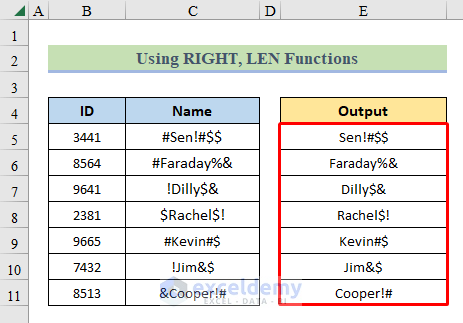
1.2 – Combining the RIGHT, and LEN Functions

This formula removes characters from the right side of the text.

Steps:

• Select cell E5 and enter the formula below:

Where,

• The LEN function provides the length of the texts.
• The RIGHT function returns a specific number of characters in the text, counting from the right.

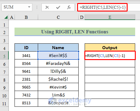
• Press ENTER and drag the “Fill Handle” down to fill the rest of the cells in Output.

All the special characters from the right are removed.

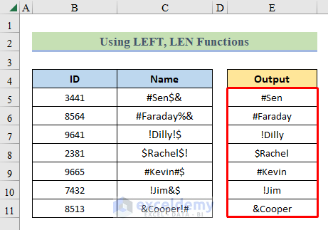
1.3 Using the LEFT and LEN Functions

You can similarly remove a special (or any other) character from the left of the text with the help of the LEFT and LEN functions.

Steps:

• Select cell E5 and enter the following formula:

Where,

• The LEN function returns the length of the string.
• The LEFT function then removes 2 characters from the left and provides an output of #Sen.

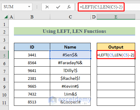
• Press ENTER  and pull the “Fill Handle” down to fill the column.

All the special characters are removed from the left.

Method 2 – Using the Flash Fill Feature

The Flash Fill is the easiest way to remove special characters in Excel.

Steps:

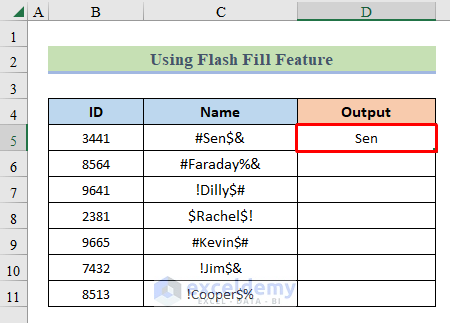
• Select cell D5 and type “Sen” (the text in cell C5 without the special characters).

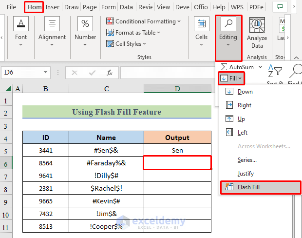
• Select cell D6.
• Go to the Home Ribbon.
• Click Editing >> Fill >> Flash Fill

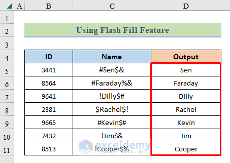
The Excel Flash Fill feature will automatically fill the other cells in the column without special characters.

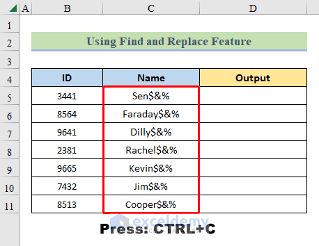
Method 3 – Using the Find & Replace Feature

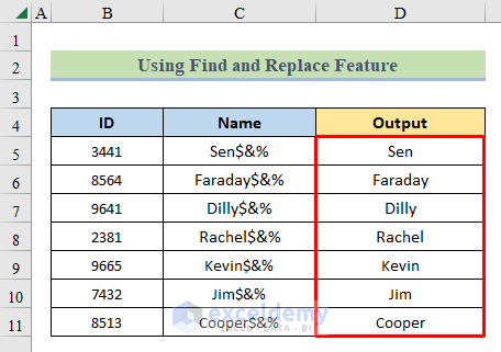
Let’s erase the special characters from the Name column below, and return the “clean” names in a new column.

Steps:

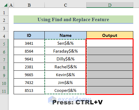
• Select cells C5:C11 and press CTRL+C to copy.

• Select cells D5:D11 and hit CTRL+V to paste.

• Select the pasted output.
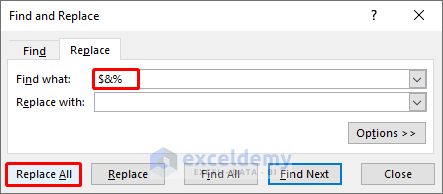
• Use the keyboard shortcut CTRL+F to open the Find and Replace window.

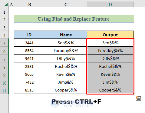
• In the “Find what” box, enter the special characters “$&%” and leave the “Replace with” box blank.
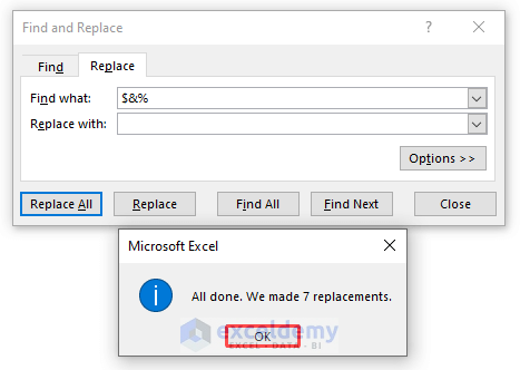
• Click “Replace All”.

A confirmation window will pop up confirming all the replacements.

The names without the special characters are successfully extracted.

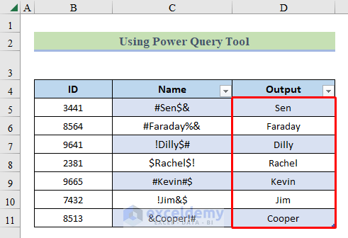
Method 4 – Using the Power Query Tool

If you are using Microsoft Excel 2016 or Excel 365, the Power Query tool is pre-installed. If you are using Microsoft Excel 2010 or 2013, you can install it from the Microsoft website.

Steps:

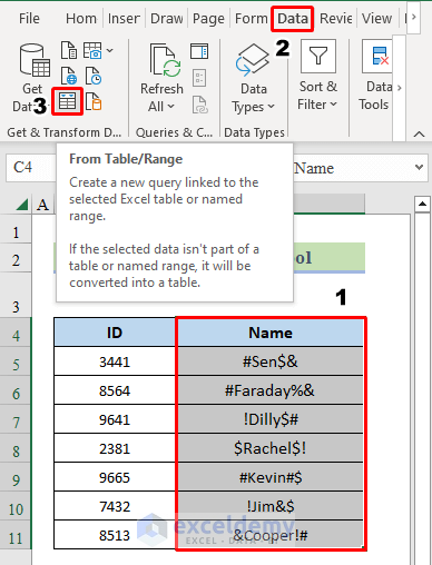
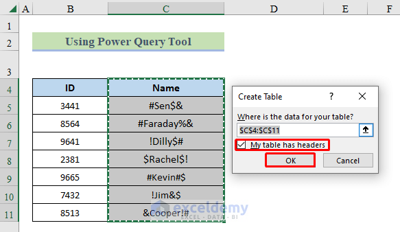
• Select your range of data along with the header.
• Select From Table/Range from the Data tab.

A “Create Table” dialog box will open.

• Select the range of your selected data and tick My table has headers.
• Click OK.

A new window named Power Query Editor will open.

• Select Custom Column from the Add Column tab.

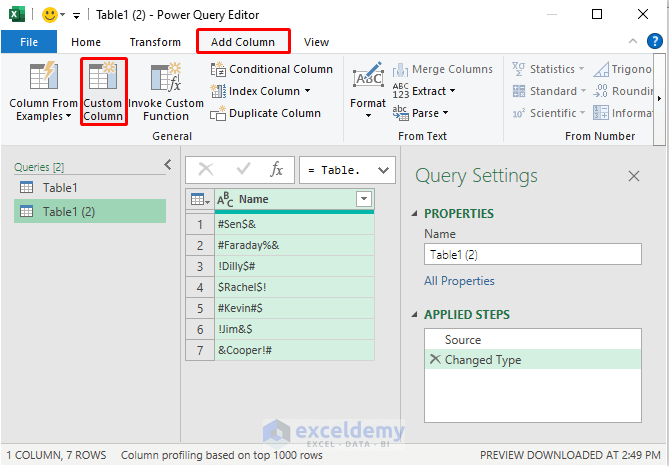
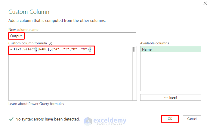
The Custom Column box will open.

• Enter “Output” as the New column name option (or whatever name you want).
• Enter the formula below in the Custom column formula field:

• Click the OK button.

• Click Close & Load from the File tab of the Power Query Editor.

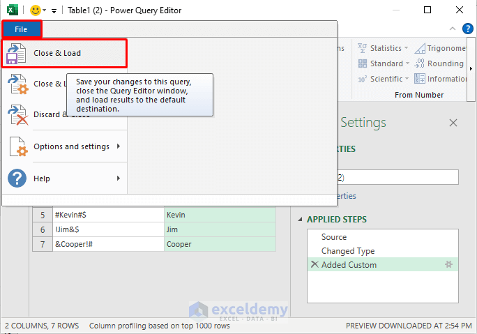
You will find a new worksheet in your workbook where you will see the final result as shown here.

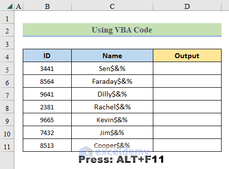
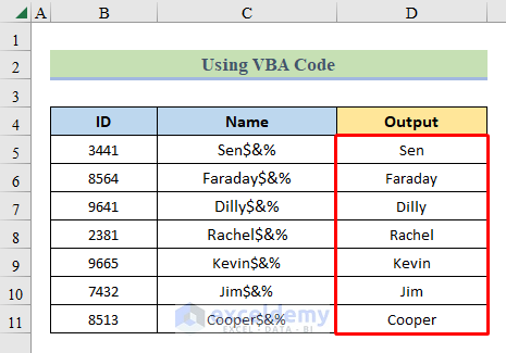
Method 5 – Using VBA Code

In this VBA code, we will define a user-defined function to remove special characters, and then apply it.

Steps:

• Open the worksheet and press ALT+F11 to open the “Microsoft Visual Basic for applications” window.

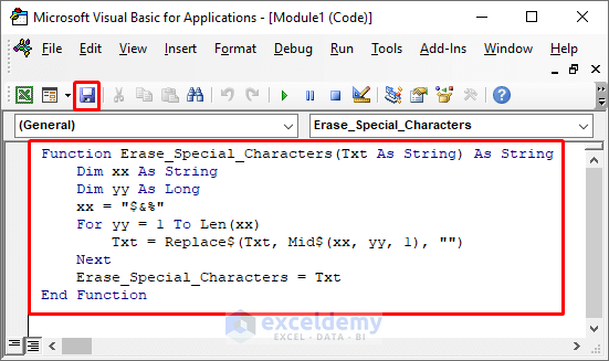
• Inside the new module place the following code and click “Save”:

Function Erase_Special_Characters(Txt As String) As String
Dim xx As String
Dim yy As Long
xx = "$&%"
For yy = 1 To Len(xx)
Txt = Replace$(Txt, Mid$(xx, yy, 1), "")
Next
Erase_Special_Characters = Txt
End Function

• Go back to the worksheet.
• Select cell D5 and enter the below formula:

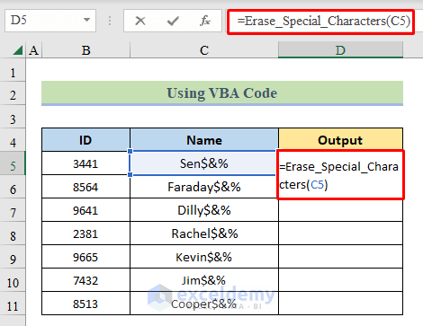
• Press ENTER and drag the “Fill Handle” down to fill the column.

All the special characters are removed from the cells.

Read More: How to Remove Characters from String Using VBA in Excel

Things to Remember

• When using the Flash Fill feature to fill cells, the columns or rows to fill from/to must be adjacent to each other.
• If you are using Microsoft Excel versions older than 2010, you might not be able to install Power Query.
• All the methods have pros and cons, so use what is appropriate for your requirements.

Download Practice Workbook

Related Articles

• How to Remove Characters from Left in Excel
• How to Remove Characters from Left and Right in Excel
• How to Remove Numeric Characters from Cells in Excel
• How to Remove Non-numeric Characters from Cells in Excel
• How to Remove Characters After a Specific Character in Excel
• Excel Remove Characters From Right

<< Go Back To Excel Remove Characters | Data Cleaning in Excel | Learn Excel