How to Remove Characters from Left in Excel (6 Methods)

Method 1 – Using the REPLACE Function

• The REPLACE function allows us to replace characters within a text string.
• The basic syntax of the REPLACE function is as follows:

=REPLACE(string, start_position, num_chars, new_text)

• • string: The original text.
  • start_position: The position from which to start replacing characters (1 for the leftmost character).
  • num_chars: The number of characters to replace.
  • new_text: The replacement text (in our case, an empty string to remove characters).

• Step-by-Step Instructions:
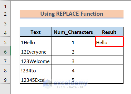
  • In cell D5, enter the following formula:

• • • This formula will remove the specified number of characters from the left side of the value in cell B5.

• • Press Enter to apply the formula.

• • Drag the Fill Handle (the small square at the bottom right corner of the cell) over the range of cells D6:D9 to apply the same operation to other values.

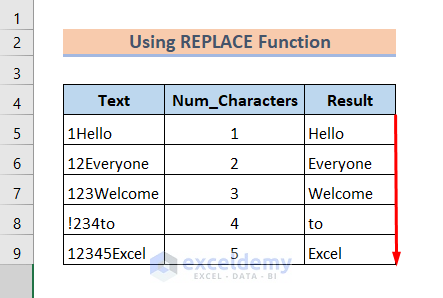
As a result, you’ll see that the specified characters have been removed from the left side of each value.

Method 2 – Using the RIGHT and LEN Functions

The RIGHT and LEN functions are commonly used to manipulate text in Excel. In this case, we’ll leverage the RIGHT function to delete characters from the left side of a text value.

Formula Syntax:

=RIGHT(text,LEN(text)-num_chars)

• Step-by-Step Instructions:
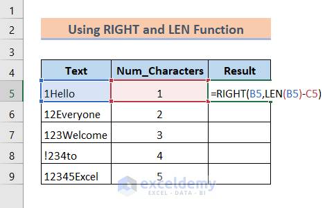
  • In cell D5, enter the following formula:

• • Explanation:
    • B5: Refers to the original text value in cell B5.
    • LEN(B5) – C5: Calculates the number of characters to remove from the left side.

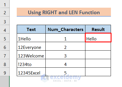
• • Press Enter to apply the formula

• • Drag the Fill Handle (located at the bottom right corner of the cell) over the range of cells D6:D9 to apply the same operation to other values.

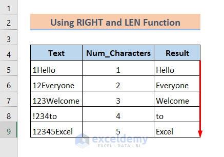
As a result, the specified number of characters will be removed from the left side of each value.

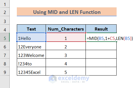
Method 3 – The MID and LEN Functions

The MID function in Excel allows us to extract a portion of text from within a larger text string. In the context of removing characters from the left side of a value, the MID function will help us achieve this automatically.

Formula Syntax:

=MID(text,1+num_chars,LEN(text))

Here’s how it works:

• text : Refers to the original text value.
• 1 + num_chars : Specifies the starting position for extracting characters (excluding the leftmost character we want to remove).
• LEN(text) : Determines the total length of the original text.

• Step-by-Step Instructions:
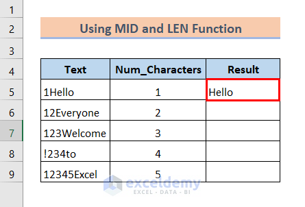
  • In cell D5, enter the following formula:

• • • Explanation:
      • B5 : Represents the original text value in cell B5.
      • 1 + C5 : Defines the starting position for extraction.
      • LEN(B5) : Calculates the total length of the original text.

• • Press Enter to apply the formula.

• • Drag the Fill Handle (located at the bottom right corner of the cell) over the range of cells D6:D9 to apply the same operation to other values.

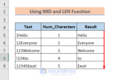
As a result, the specified characters will be removed from the left side of each value.

Method 4 – Using the SUBSTITUTE Function

Unlike the other methods, we’ll utilize the SUBSTITUTE function to replace specific characters from the left side of a text value with an empty string.

Formula Syntax:

=SUBSTITUTE(Text,LEFT(Text,num_chars),””)

In this case, the LEFT function will return the characters from the left that we want to delete.

Here’s how it works:

• Text : Refers to the original text value.
• LEFT(Text, num_chars) : Extracts the leftmost characters (up to the specified number) that we want to delete.
• The SUBSTITUTE function then replaces these extracted characters with an empty string.

• Step-by-Step Instructions:
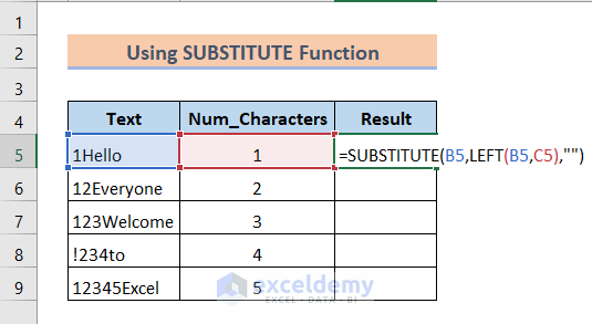
  • In cell D5, enter the following formula:

• • Explanation:
    • B5 : Represents the original text value in cell B5.
    • LEFT(B5, C5) : Retrieves the leftmost characters up to the specified count (C5).

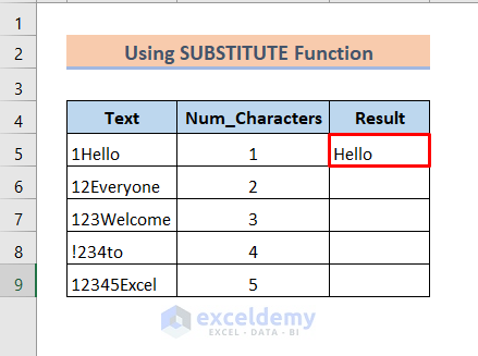
• • Press Enter to apply the formula.

• • Drag the Fill Handle (located at the bottom right corner of the cell) over the range of cells D6:D9 to apply the same operation to other values.

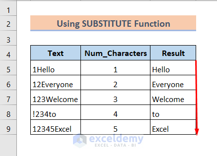
As a result, the specified characters will be removed from the left side of each value.

Method 5 – Using Text to Columns to Split and Remove Characters from the Left in Excel

The Text to Columns feature in Excel allows us to split data within a single column into multiple columns based on specific criteria. In this case, we’ll demonstrate how to split and remove characters from the left side of a dataset using this method.

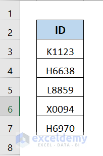
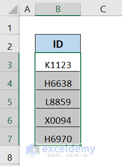
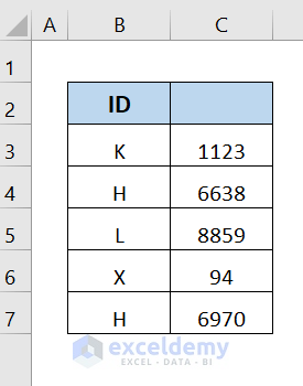
• Dataset Description:
  • We have a dataset with a single column (B3:B7) containing text values.
  • Our goal is to split the text based on a specific character position (from the left).

• Step-by-Step Instructions:
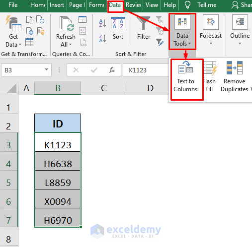
  • Select the range of cells B3:B7 that contains your data.
  • Navigate to the Data tab in the Excel ribbon.
  • Under Data Tools, click on Text to Columns.

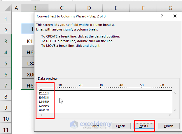
• • In the dialog box that appears:
    • Choose the Fixed width option and click Next.

• • • Define the positions where you want to split the text. For example, if you want to split after the first character, select the space between the first and second characters.

• • • Click Next.
    • Review the preview to ensure the correct split positions.

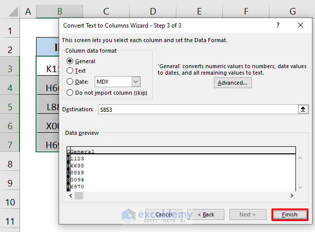
• • • Click Finish.

As a result, your data will be divided into separate columns based on the specified character position (from the left).

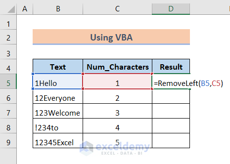
Method 6 – Using Excel VBA to Remove Characters from the Left

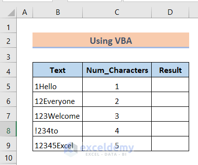
We are using this dataset to demonstrate this method:

• Open your Excel workbook.
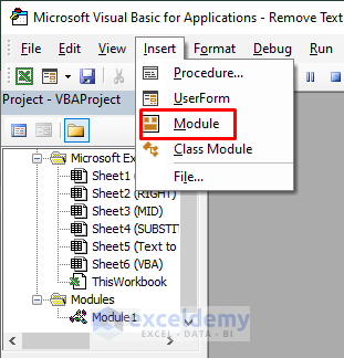
• Press Alt+F11 on your keyboard to open the Visual Basic for Applications (VBA) editor.
• In the VBA editor, click Insert > Module to create a new module.

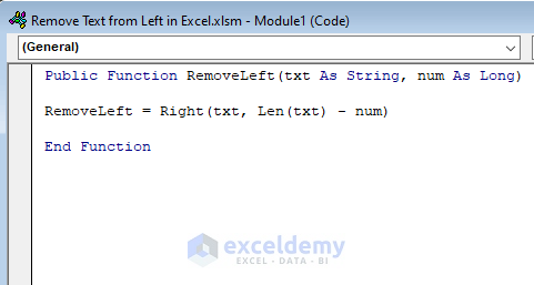
• Copy and paste the following VBA code into the module:

Public Function RemoveLeft(txt As String, num As Long)
RemoveLeft = Right(txt, Len(txt) - num)
End Function

• Return to your dataset in Excel.
• In cell D5, enter the following formula:

=RemoveLeft(B5,C5)

Replace B5 with the cell containing the original text and C5 with the number of characters you want to remove from the left.

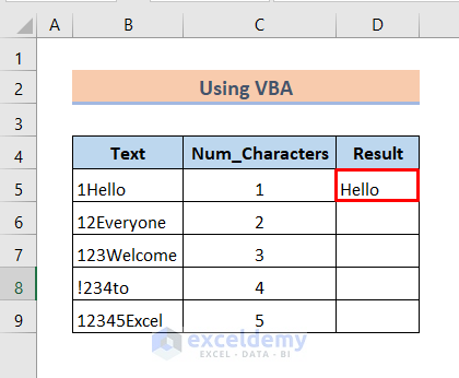
• Press Enter.

• Drag the fill handle over the range of cells D6:D9 to apply the formula to the entire column.

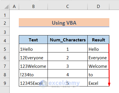
You’ll see that characters have been successfully removed from the left using VBA.

Download Practice Workbook

You can download the practice workbook from here:

Excel Remove Characters from Left: Knowledge Hub

• Remove First Character in Excel
• Remove First 3 Characters in Excel
• Remove the First Character from a String in Excel with VBA
• Remove Characters from Left and Right in Excel

<< Go Back To Excel Remove Characters | Data Cleaning in Excel | Learn Excel