How to Use RIGHT Function in Excel (6 Suitable Examples)

RIGHT is another popular function in MS Excel that is used to get the last character or characters in a text string, based on the specific number of characters. In one word, this function is designed to return a specified number of characters from the rightmost side of a string. This article will share a complete idea of how the RIGHT function works in Excel independently and then with other Excel functions.

RIGHT Function in Excel (Quick View)

Excel RIGHT Function


Introduction to RIGHT Function in Excel

  • Objective

To extract a specified number of characters from a given string from right to left.

  • Syntax
=RIGHT (text, [num_chars])
  • Arguments Explanation
Arguments Required/Optional Explanation
text Required Pass the text from which to extract characters on the right.
[num_chars] Optional Pass the number of characters to extract, starting on the right. The default value is 1.
  • Available in

The RIGHT function is available from Excel 2007 to Present version.

Notes
  • If num_chars is not provided, it defaults to 1.
  • If num_chars is greater than the number of characters available, the RIGHT function returns the entire text string.
  • RIGHT will extract digits from numbers as well as text.
  • This function does not consider the formatting of any cell. Like a date, currency, etc.
  • While writing this article, I’m using the Office 365.

How to Use the RIGHT Function in Excel: 6 Suitable Examples

In the following sections, we will demonstrate six examples for describing the RIGHT function. We will apply the RIGHT function, LEN, SEARCH, SUBSTITUTE, VALUE, and FIND functions as well in these examples for substring operation with space, delimiter, and n characters. In addition, we will extract numbers and domains from the string and modify the URL by using the RIGHT function.


Example 1: Using RIGHT Function to Get a Substring Until Space

Let’s assume we have a dataset of customers with their Names, Order IDs, Addresses, and Total Prices. Now we will extract the last name of each customer from their full name using the RIGHT function. Let’s follow the instructions below to learn!

Step 1:

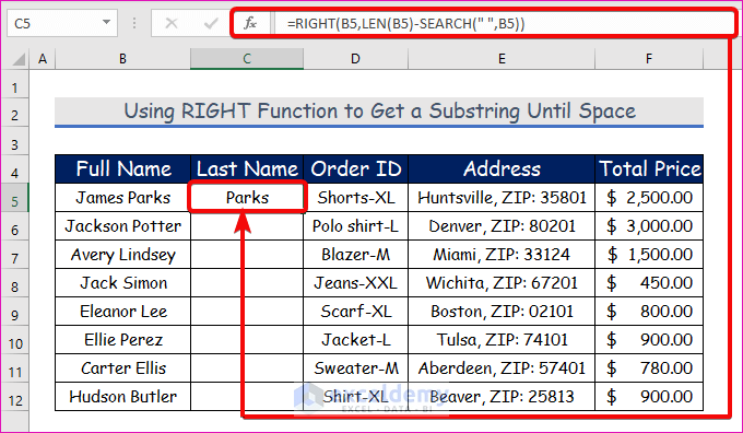
  • Write down the below formula in cell C5.
=RIGHT(B5,LEN(B5)-SEARCH(" ",B5))
Formula Breakdown
  • SEARCH(" ", B5) this portion finds the space from the Full name cells.
  • Then LEN(B5)-SEARCH(" ", B5) this portion will select the last part of the name.
  • Then the RIGHT function will return the selected portion.
  • Hence, simply press Enter on your keyboard. As a result, you will get Parks as the return of the RIGHT function.
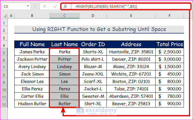
Using RIGHT Function to Get a Substring Until Space

Step 2:

  • Further, AutoFill the RIGHT function to the rest of the cells in column C.


Example 2: Extract a Substring Using the RIGHT, LEN, SEARCH, and SUBTITUTE Functions

Now consider that we have a dataset of customer comments. In each comment, there is a comment number like Comments 1, Comments 2, etc. Now our task is to extract the only comments from the source comment. Let’s follow the instructions below to learn!

Steps:

  • Enter the formula in cell D5 and AutoFill it up to D12.
=RIGHT(C5,LEN(C5)-SEARCH("$",SUBSTITUTE(C5,":","$",LEN(C5)-LEN(SUBSTITUTE(C5,":","")))))

Formula Breakdown

  • LEN(SUBSTITUTE(C5,":","")) this portion finds the colon (:) sign in the whole string.
  • SUBSTITUTE(C5,":","#",LEN(C5)-LEN(SUBSTITUTE(C5,":",""))) this part replaces the last delimiter with some unique character.
  • Then SEARCH("#", SUBSTITUTE(C5,":","#",LEN(C5)-LEN(SUBSTITUTE(C5,":","")))) this part gets the position of the last delimiter in the string. Depending on what character we have replaced the last delimiter with, use either case-insensitive SEARCH or case-sensitive FIND to determine the position of that character in the string.
  • Lastly, the RIGHT function selects comments and prints them.
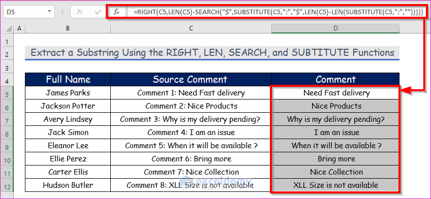

Example 3: Remove First N Characters from a String Applying RIGHT Function

The above task can be done using a simple formula. As there is a fixed number of characters in “Comment N” which is 10 in the first portion of each comment, we can easily eliminate it and get the comment only. Here we will remove the first 10 characters from the Source Comment and print the only comments in a separate column. Let’s follow the instructions below to learn!

Steps:

  • First of all, select cell D5, and Enter the formula in that cell. After that, AutoFill it up to D12.
=RIGHT(C5, LEN(C5)-10)
Formula Explanation
  • LEN(C5)-10 this will return a number after subtracting 10 from the total characters number. If the total length is 25 then this portion will return 25-10 = 15.
  • Then the RIGHT function will return the only comment from the source comment.
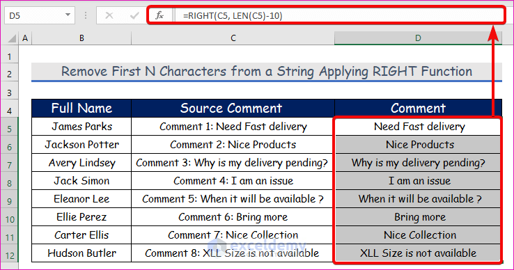
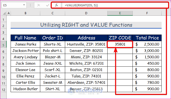
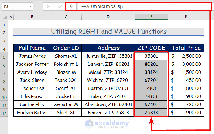
Remove First N Characters from a String Applying RIGHT Function


Example 4: Utilizing RIGHT and VALUE Functions to Extract Number from a String

The RIGHT function does not allow the return of a number from any string. It returns the number in text format. But using the VALUE and RIGHT functions, we can return numbers in the correct format. Here we will use the same dataset as above, and we will extract the ZIP Code in number format from the Address column. Let’s follow the instructions below to learn!

Step 1:

  • Write down the below formula in cell E5.
=VALUE(RIGHT(D5, 5))
Formula Explanation
  • RIGHT(D5, 5) this portion gives the 5 characters from the address which is the zip code in text format.
  • Then VALUE function converts them into a number format.
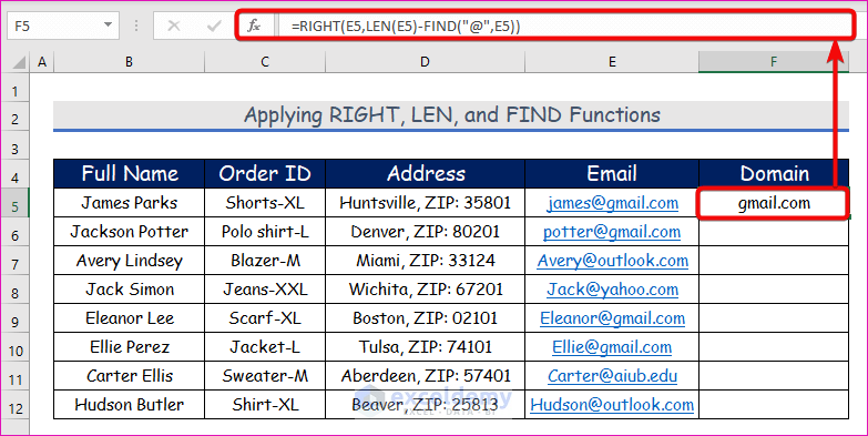
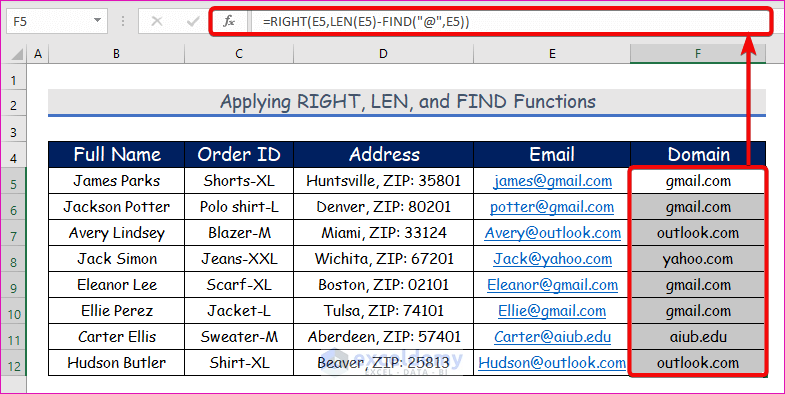
  • After that, simply press Enter on your keyboard. Hence, you will get 35801 as the return of the functions.

Utilizing RIGHT and VALUE Functions to Extract Number from a String

Step 2:

  • Further, AutoFill the functions to the rest of the cells in column E.


Example 5: Applying RIGHT, LEN, and FIND Functions to Extract Domain Name from Email

Let’s have a customer dataset with their Order ID, Name, Email, and Address. Now we will find out their email domain from the given email address using the RIGHT, LEN, and FIND functions. Let’s follow the instructions below to learn!

Step 1:

  • First of all, select cell F5, and write down the below formula in that cell.
=RIGHT(E5,LEN(E5)-FIND("@",E5))
Formula Explanation
  • FIND("@",E5) this portion finds @ from the given string.
  • LEN(E5)-FIND("@", E5) this will give the number up to which the value will be extracted.
  • Hence, simply press Enter on your keyboard. As a result, you will get gmail.com as the return of the RIGHT, LEN, and FIND functions.

Applying RIGHT, LEN, and FIND Functions to Extract Domain Name from Email

Step 2:

  • After that, AutoFill the RIGHT, LEN, and FIND functions to the rest of the cells in column F.


Example 6: Using RIGHT, LEN, and LEFT Functions to Modify URL

This RIGHT function also helps us modify any type of URL. Let’s say that in our dataset we have several URLs of some websites. Now, in some of them, there is a backslash(/) in the URL. Now our task is to find out those URLs and remove this backslash from the URL. Let’s follow the instructions below to learn!

Steps:

  • Enter the formula in cell C5 and AutoFill it up to C9.
=LEFT(B5,LEN(B5)-(RIGHT(B5)="/"))
Formula Explanation
  • If the last character is a forward slash (/), (RIGHT(B5)=”/”) returns “true,” or else it returns “false”.
  • The =LEFT(B5, LEN(B4)-(RIGHT(B5)=”/”)) returns the first “n” number of characters. If the last character is a forward slash (/), it is omitted; else, the complete string is returned.

Using RIGHT, LEN, and LEFT Functions to Modify URL


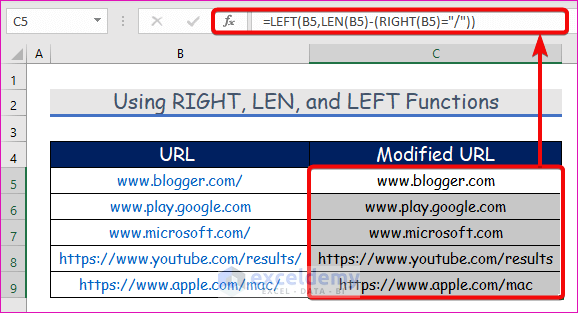
Special Notes for Using RIGHT Function of MS Excel

  • Does the RIGHT function return number?
    The RIGHT function in Excel always produces a text string, despite the fact that the initial value was a number, as was stated at the beginning of this lesson.
  • The RIGHT function can not work with dates?
    Since dates are represented by integers in the internal Excel system and the Excel RIGHT function is built to operate with text strings, it is not possible to extract a specific part of a date, such as a day, month, or year. If you try this, all you will receive are the final few digits of a number that represents a date.
  • Why the RIGHT function returns #VALUE error?
    The RIGHT function returns #VALUE! error if “num_chars” is less than zero.

Download Practice Workbook

Download this practice workbook to exercise while you are reading this article.


Conclusion

That’s all about the RIGHT function. Here I have tried to give a summary of this function and its different applications. I have shown multiple methods with their respective examples, but there can be many other iterations depending on numerous situations. If you have any inquiries or feedback, please let us know in the comment section.


<< Go Back to Excel Functions | Learn Excel

Get FREE Advanced Excel Exercises with Solutions!
Md. Abdullah Al Murad

Md. Abdullah Al Murad is a computer engineer who loves exploring Excel and VBA programming. Programming, to him, is a time-saving tool for efficiently managing data, files, and internet tasks. He is proficient in C, C++, Python, JavaScript, HTML, SQL, MySQL, PostgreSQL, Microsoft Office, and VBA and goes beyond the basics. He holds a B.Sc. in Computer Science and Engineering from American International University-Bangladesh. He has transitioned into the role of a content developer. Beyond his work, find... Read Full Bio

2 Comments
  1. Reply
    Nohemi West-Phelps Dec 23, 2021 at 5:20 AM

    Hi – I am trying to write a formula to extract the name and address from these strings. My thought was to try to do an IF statement since they either start with PRM-OC-SF-Note or PRM-SF-Deed of Trust. Something like IF cell = “PRM-OC-SF-Note” then remove the first 42 characters but IF cell = “PRM-SF-Deed of Trust” then remove the first 53 characters. Then I can do a comma delimited for the rest. But I am not sure how to combine and IF function with a Left/Right trim. Also not sure if there is a better formula
    Client Column
    PRM-OC-SF-Note – 5/28/2010 – 0001111111- DOE – JANE – 111 WINDY AVE – SINGLE FAMILY – OMITTED – – – – -144444444
    PRM-SF-Deed of Trust – 11/11/2008 – 0001111111 – DOE – JANE – 111 WINDY AVE – SINGLE FAMILY – – – – – – -1444444444
    PRM-OC-SF-Note – 8/18/2008 – 0033333333 – DOE – JIM – 1222 OXFORD CIR – SINGLE FAMILY – – – – – -1433333333
    PRM-SF-Deed of Trust – 7/1/2008 – 0033333333 – DOE – JIM – 1222 OXFORD CIR – SINGLE FAMILY – PAID OFF – – – – – 1593-1433333333
    PRM-OC-SF-Note – 9/15/2009 – 0034444444- SMITH – JOHN – 333 ELMWOOD PKWY – GINNIE MAE – SECURITIZED – 0222222222 – 0000000000 – 11/3/2009 – 5/20/2010-1455555555
    PRM-SF-Deed of Trust – 7/8/2014 – 0034444444- SMITH – JOHN – 333 ELMWOOD PKWY – GINNIE MAE – SECURITIZED – 0222222222 – – – – -1455555555

Leave a reply

Advanced Excel Exercises with Solutions PDF


ExcelDemy
Logo