Dataset Overview
In large datasets, duplicate values or repeated occurrences of the same values can be a common issue. To address this, you can utilize the Excel UNIQUE function, which returns a list of unique values from a specified range or list. Whether dealing with text, numbers, dates, or times, the UNIQUE function is versatile and helpful.
Basics of EXP Function – Summary & Syntax
Summary
The Excel UNIQUE function identifies and extracts unique values within a given range or list. It allows you to obtain both strictly unique values and distinct values (where duplicates are removed). Additionally, it facilitates comparisons between columns or rows.
Syntax
The UNIQUE function has the following syntax:
UNIQUE(array, [by_col], [exactly_once])
- array: The range or list from which you want to extract unique values.
- by_col (optional): If set to TRUE, the function treats the array as columns; if FALSE (or omitted), it treats the array as rows.
- exactly_once (optional): If TRUE, only values occurring exactly once are considered unique; if FALSE (or omitted), all unique values are returned.
Return Value
The UNIQUE function provides a list or array containing the unique values.
Version Compatibility
The UNIQUE function is available for Excel 365 and Excel 2021.
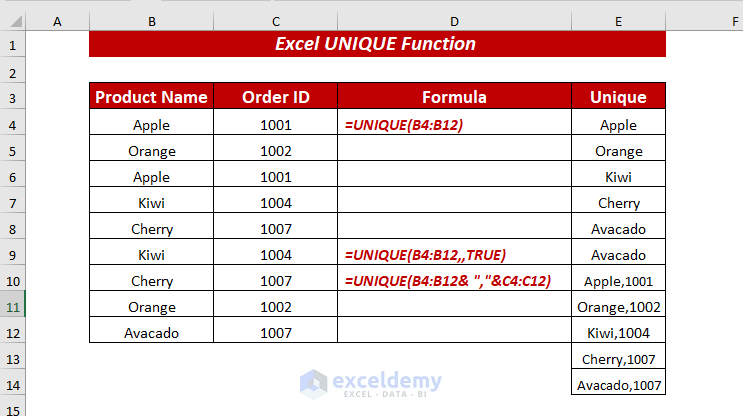
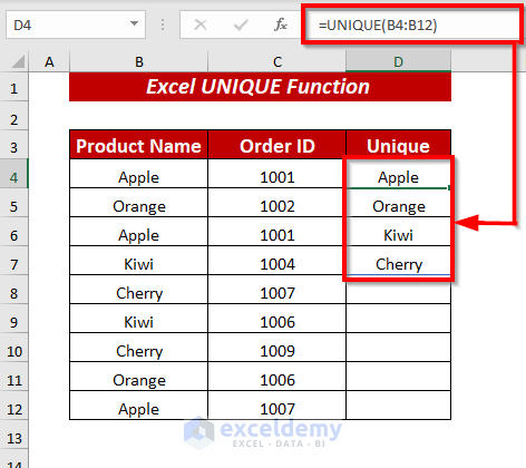
Example 1 – Extracting Unique Text Values
Suppose you have a column named Product Name containing various fruit names. To obtain the unique fruit names, follow these steps:
- In cell D4, enter the following formula:
=UNIQUE(B4:B12)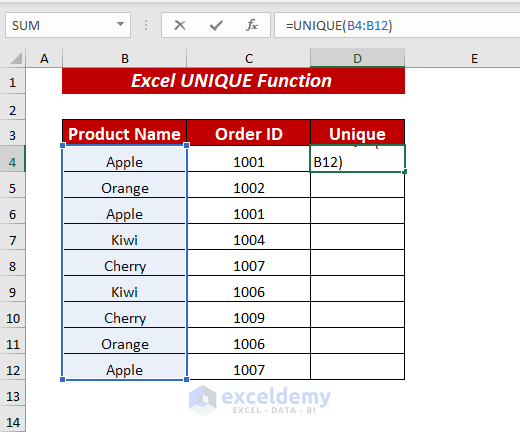
- Press ENTER, and the UNIQUE function will return the list of unique fruit names from the specified range (B4:B12).
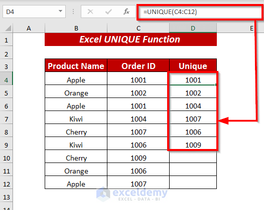
Example 2 – Extracting Unique Numeric Values
If you’re working with numeric values, such as order IDs, you can still use the UNIQUE function. For instance:
- In cell D4, enter the following formula:
=UNIQUE(C4:C12)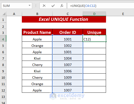
- Press ENTER, and the UNIQUE function will provide the list of unique order IDs from the specified range (C4:C12).
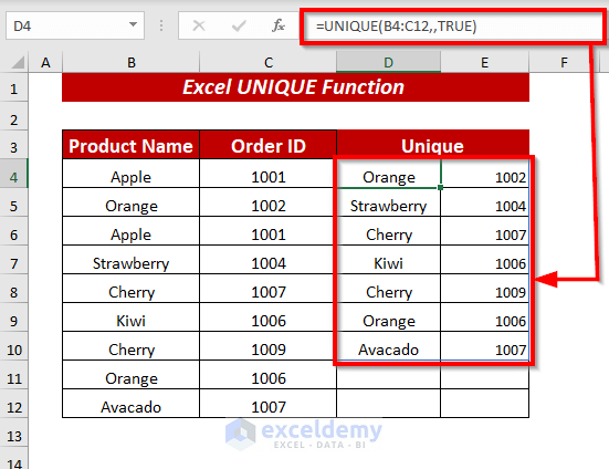
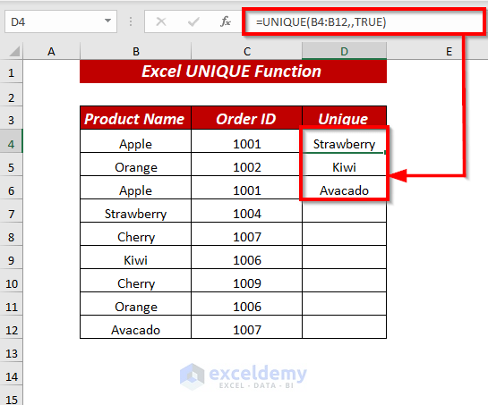
Example 3 – Finding Unique Rows Occurred Only Once
If you need to identify unique values that occurred only once within a list or range, the UNIQUE function can help. Follow these steps:
- In cell D4, enter the following formula:
=UNIQUE(B4:C12,,TRUE)-
- Here, we selected the cell range B4:C12 as an array.
- We kept the by_col argument as FALSE (or omitted it) because the dataset is organized in rows.
- We set exactly_once to TRUE.
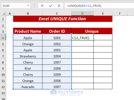
- Press ENTER, and the UNIQUE function will return the list of unique values that occurred only once from the selected range.
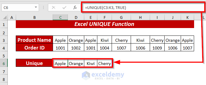
Example 4 – Extracting Unique Values from a Row
To obtain unique values from a row, follow these steps:
- In cell C6, enter the following formula:
=UNIQUE(C3:K3, TRUE)-
- Here, we selected the cell range C3:K3 as an array.
- We set by_col to TRUE.
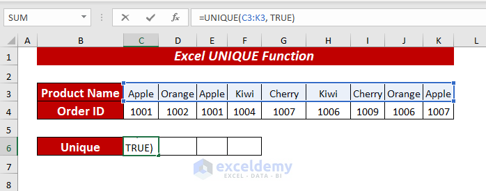
- Press ENTER, and the UNIQUE function will return the unique values from the row.
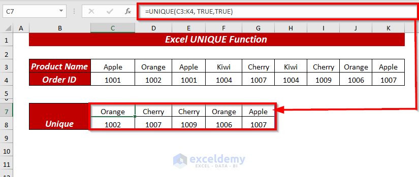
Example 5 – Finding Unique Columns Using the UNIQUE Function
You can also extract unique columns using the UNIQUE function:
- In cell C7, enter the following formula:
=UNIQUE(C3:K4, TRUE,TRUE)- Here, we selected the cell range C3:K4 as an array.
- We set by_col to TRUE.
- We also set exactly_once to TRUE.
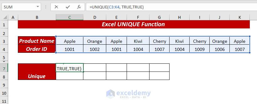
- Press ENTER, and the UNIQUE function will return the unique columns.
Example 6 – Extracting Unique Values from a List
If you want to extract unique values from a list, follow these steps:
- In cell D4, enter the following formula:
=UNIQUE(B4:B12,,TRUE)- Here, we selected the cell range B4:B12 as an array.
- We kept the by_col argument as FALSE (or omitted it) because the dataset is organized in rows.
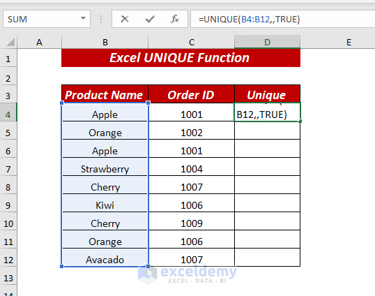
Press ENTER, and the UNIQUE function will return the list of unique values that occurred only once from the selected range.
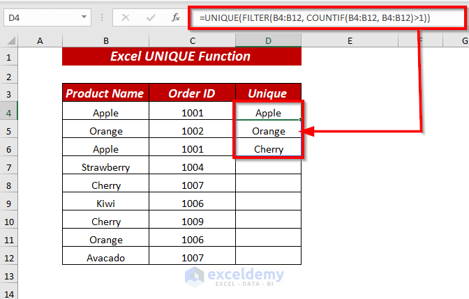
Example 7 – Finding Distinct Values That Occur More Than Once
To identify distinct unique values that occur more than once, you can combine the UNIQUE function with the FILTER function and the COUNTIF function. Follow these steps:
- In cell D4, enter the following formula:
=UNIQUE(FILTER(B4:B12, COUNTIF(B4:B12, B4:B12)>1))-
- In the UNIQUE function, we used FILTER(B4:B12, COUNTIF(B4:B12, B4:B12)>1) as an array.
- In the FILTER function, we selected the range B4:B12 as an array and used COUNTIF(B4:B12, B4:B12)>1) as the inclusion criteria.
- The COUNTIF function counts the occurrences of values greater than 1 (i.e., those occurring more than once).
- The UNIQUE function returns the distinct values that occurred more than once.
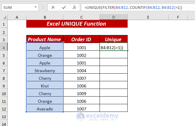
- Press ENTER, and the UNIQUE function will provide the unique values occurring more than once.
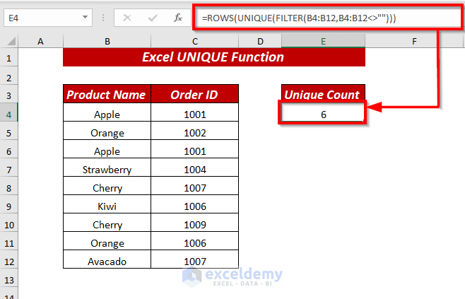
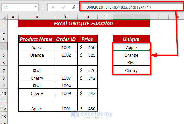
Example 8 – Counting Unique Values Using the Excel UNIQUE Function
You can also count the unique values by combining the FILTER function with the ROWS function:
- In cell D4, enter the following formula:
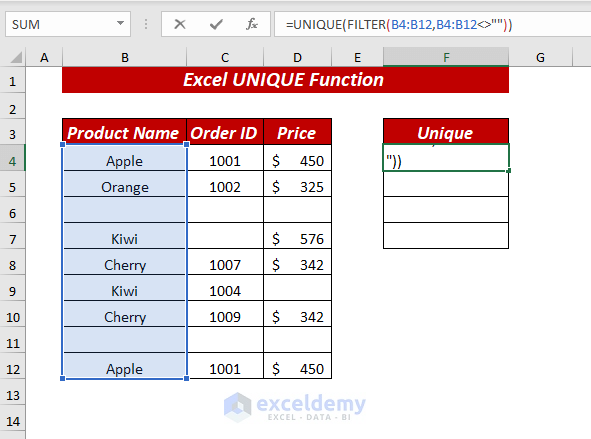
=ROWS(UNIQUE(FILTER(B4:B12,B4:B12<>"")))-
- In the ROWS function, we used UNIQUE(FILTER(B4:B12,B4:B12<>””)) as an array.
- In the UNIQUE function, we used FILTER(B4:B12,B4:B12<>””) as an array.
- In the FILTER function, we selected the range B4:B12 as the array and filtered out blank values (i.e., not equal to blank).
- The UNIQUE function returns the unique values from the filtered list, and the ROWS function calculates the count of unique values.
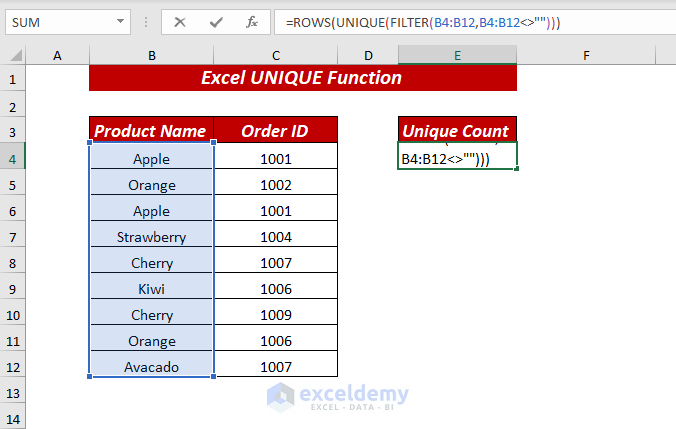
- Press ENTER, and you’ll obtain the count of unique values.
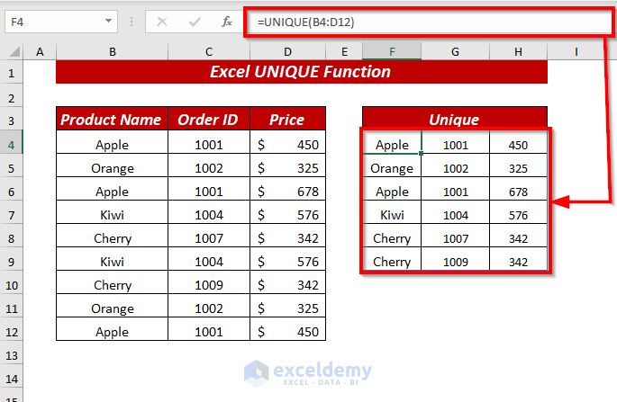
Example 9 – Unique Values From Multiple Columns
If you want, you can extract unique values from multiple columns as well, just by using the UNIQUE function.
- In cell F4, insert the following formula to get the unique values from multiple columns.
=UNIQUE(B4:D12)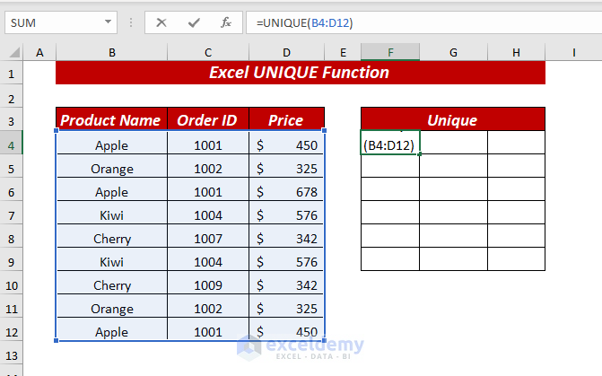
Here, in the UNIQUE function, we selected the cell range B4:D12 as an array.
- Press ENTER, and the UNIQUE function will return the range of unique values from multiple columns.
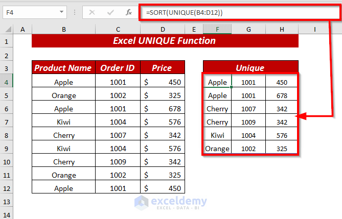
Example 10 – Sorting Unique Values Sorting in Alphabetical Order
To sort unique values alphabetically, you can combine the UNIQUE function with the SORT function. Follow these steps:
- In cell F4, enter the following formula:
=SORT(UNIQUE(B4:D12))-
- Here, we selected the cell range B4:D12 as an array in the UNIQUE function.
- The UNIQUE function extracts the unique values from the specified columns.
- The SORT function then sorts these unique values alphabetically.

- Press ENTER, and you’ll obtain the sorted unique values from the multiple columns.
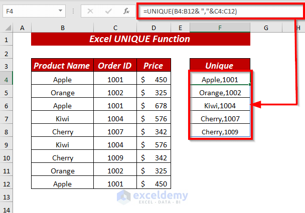
Example 11 – Concatenating Unique Values from Multiple Columns into One Cell
If you want to extract unique values from multiple columns and concatenate them into a single cell, follow these steps:
- In cell F4, enter the following formula:
=UNIQUE(B4:B12& ","&C4:C12)-
- Here, we selected both cell ranges B4:B12 and C4:C12 as an array.
- The UNIQUE function extracts the unique values from both column ranges.
- The concatenation operator (&) combines these unique values with a comma (,).
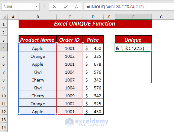
- Press ENTER, and you’ll get the concatenated values in one cell.
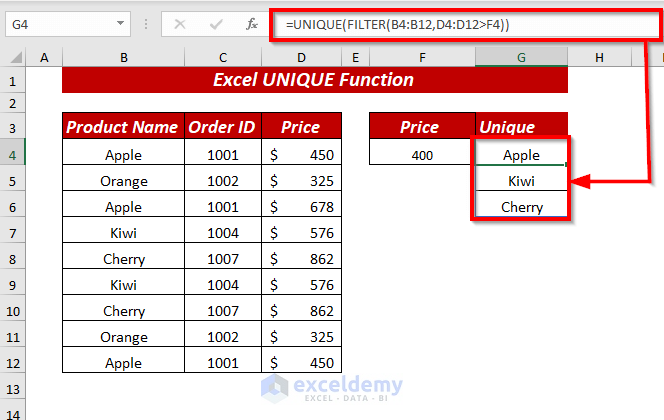
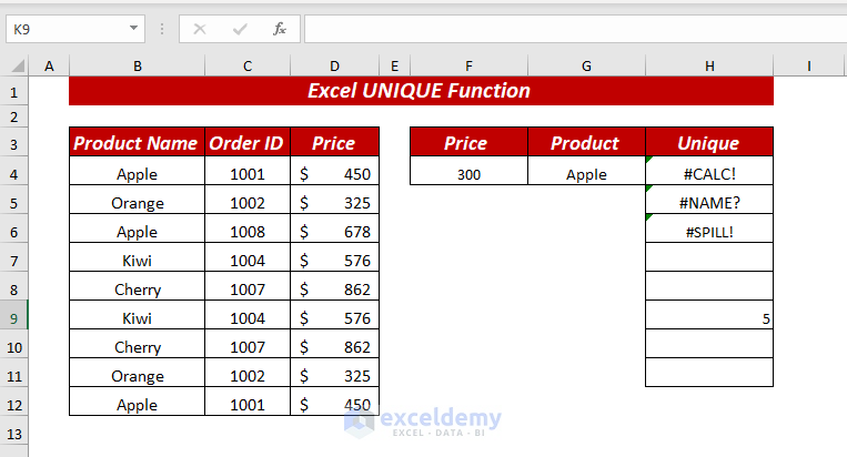
Example 12 – List of Unique Values Depending on Criteria
If you want to get the list of unique values based on criteria using the UNIQUE function along with the FILTER function, follow these steps:
- Open your Excel workbook.
- Navigate to cell G4.
- Enter the following formula to get the unique values based on criteria:
=UNIQUE(FILTER(B4:B12,D4:D12>F4))In this formula:
-
- FILTER(B4:B12,D4:D12>F4) creates an array of values from column B (Price) where the corresponding value in column D (Criteria) is greater than the value in cell F4.
- The UNIQUE function then returns the unique values from this filtered array.
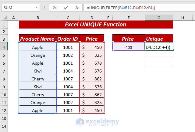
- Press ENTER to get the unique values based on your specified criteria.
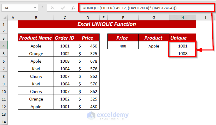
Example 13 – Filter Unique Values Based on Multiple Criteria
To extract the list of unique values based on multiple criteria using the UNIQUE function with the FILTER function, follow these steps:
- Go to cell H4.
- Enter the following formula to get the unique values based on multiple criteria:
=UNIQUE(FILTER(C4:C12, (D4:D12>F4)* (B4:B12=G4)))In this formula:
-
- FILTER(C4:C12, (D4:D12>F4)* (B4:B12=G4)) creates an array of values from column C (Product name) where both criteria are met:
- The corresponding value in column D (Price) is greater than the value in cell F4.
- The corresponding value in column B (Product name) matches the value in cell G4.
- The UNIQUE function then returns the unique values from this filtered array.
- FILTER(C4:C12, (D4:D12>F4)* (B4:B12=G4)) creates an array of values from column C (Product name) where both criteria are met:
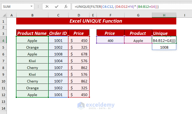
- Press ENTER to get the unique values based on your specified multiple criteria.
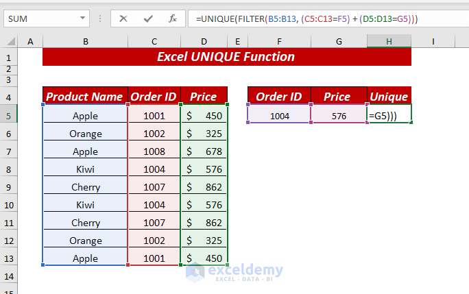
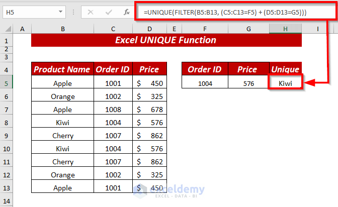
Example 14 – Filter Unique Values Based on Multiple OR Criteria
If you want, you also can use the UNIQUE and FILTER function to apply multiple OR criteria, by following these steps:
- Open your Excel workbook.
- Go to cell H4.
- Enter the following formula to get the unique values from multiple OR criteria:
=UNIQUE(FILTER(B5:B13, (C5:C13=F5) + (D5:D13=G5)))In this formula:
-
- FILTER(B5:B13, (C5:C13=F5) + (D5:D13=G5)) creates an array of values from column B (Price) where either of the following conditions is met:
- The corresponding value in column C (Criteria 1) equals the value in cell F5.
- The corresponding value in column D (Criteria 2) equals the value in cell G5.
- The UNIQUE function then returns the unique values from this filtered array.
- FILTER(B5:B13, (C5:C13=F5) + (D5:D13=G5)) creates an array of values from column B (Price) where either of the following conditions is met:
-
- Press ENTER to get the unique values based on your specified OR criteria.
Example 15 – Get Unique Values Ignoring Blanks
While using the UNIQUE function with the FILTER function you can extract unique values while ignoring blank cells, by following these steps:
- Go to cell F4.
- Enter the following formula to get the unique values while ignoring blank cells:
=UNIQUE(FILTER(B4:B12,B4:B12<>""))In this formula:
-
- FILTER(B4:B12,B4:B12<>””) creates an array of values from column B (Price) where the corresponding value is not blank (empty).
- The UNIQUE function then returns the UNIQUE from this filtered array.
- Press ENTER to get the unique values while excluding any blank cells.
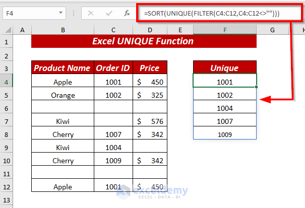
Example 16 – Using Excel UNIQUE & SORT Function to Ignore Blanks & Sort
If you want to sort the unique values while ignoring blanks by using the UNIQUE function with the FILTER function, follow these steps:
- Open your Excel workbook.
- Go to cell F4.
- Enter the following formula to get the sorted unique values while ignoring blanks:
=SORT(UNIQUE(FILTER(C4:C12,C4:C12<>"")))In this formula:
-
- UNIQUE(FILTER(C4:C12,C4:C12<>””)) creates an array of values from column C (Product name) where the corresponding value is not blank (empty).
- The UNIQUE function then returns the unique values from this filtered array.
- The SORT function sorts the unique values numerically.
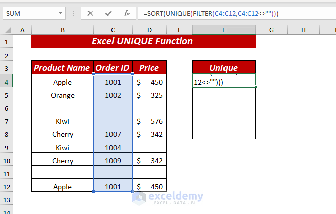
- Press ENTER to get the sorted unique values while excluding any blank cells.
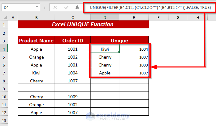
Example 17 – Using Excel UNIQUE & FILTER Function to Get Unique Rows Ignoring Blank
To get unique rows while ignoring blanks by using the UNIQUE function with the FILTER function, follow these steps:
- Go to cell D4.
- Enter the following formula to get the unique rows while ignoring blanks:
=UNIQUE(FILTER(B4:C12, (C4:C12<>"")*(B4:B12<>"")),FALSE, TRUE)In this formula:
-
- FILTER(B4:C12, (C4:C12<> “”) * (B4:B12 <> “”)) creates an array of rows from columns B and C where both conditions are met:
- The corresponding value in column C (Product name) is not blank.
- The corresponding value in column B (Price) is not blank.
- The UNIQUE function then returns the unique rows from this filtered array.
- The FALSE argument specifies that the unique rows should be returned by row (not by column).
- The TRUE argument ensures that only the first occurrence of each unique row is included.
- FILTER(B4:C12, (C4:C12<> “”) * (B4:B12 <> “”)) creates an array of rows from columns B and C where both conditions are met:
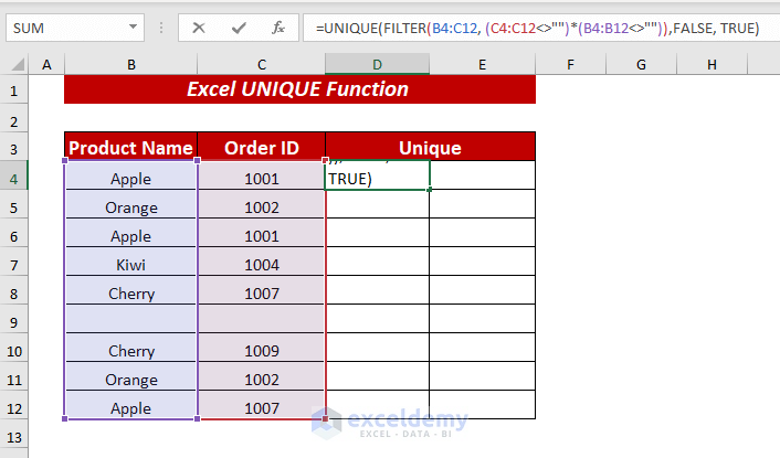
- Press ENTER to get the unique rows while excluding any blank cells.
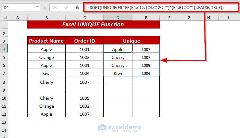
Example 18 – Filter Unique Rows Ignoring Blank & Sort
To obtain unique rows while ignoring blank cells, you can use the SORT function in conjunction with the UNIQUE and FILTER functions. This combination allows you to filter out duplicates and arrange the results in a sorted order.
- Open your Excel workbook.
- Go to cell D4.
- Enter the following formula to get the sorted unique rows while ignoring blanks:
=SORT(UNIQUE(FILTER(B4:C12, (C4:C12<>"")*(B4:B12<>"")),FALSE, TRUE))In this formula:
-
- (FILTER(B4:C12, (C4:C12<>””)*(B4:B12<>””)) creates an array of rows from columns B and C where both conditions are met:
- The corresponding value in column C (Product name) is not blank.
- The corresponding value in column B (Price) is not blank.
- The UNIQUE function then returns the unique rows from this filtered array.
- The SORT function sorts the unique rows alphabetically.
- (FILTER(B4:C12, (C4:C12<>””)*(B4:B12<>””)) creates an array of rows from columns B and C where both conditions are met:
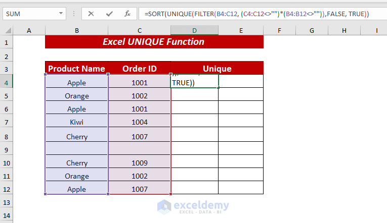
- Press ENTER to get the sorted unique rows while excluding any blank cells.
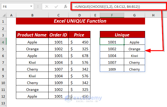
Example 19 – Using Excel UNIQUE & CHOOSE Functions to Find Unique Values in Specific Columns
To find unique values from specific columns in Excel, you can use the CHOOSE function in combination with the UNIQUE function. Here’s how:
- Go to cell D4.
- Enter the following formula to get the unique values from specific columns:
=UNIQUE(CHOOSE({1,2}, C4:C12, B4:B12))In this formula:
-
- CHOOSE({1,2}, C4:C12, B4:B12) creates an array by selecting values from columns C (Product name) and B (Price) based on the specified indices.
- The UNIQUE function then returns the unique values from this combined array.
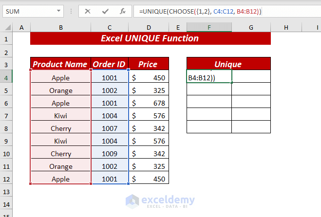
- Press ENTER to get the unique values from the selected range of the specific columns.
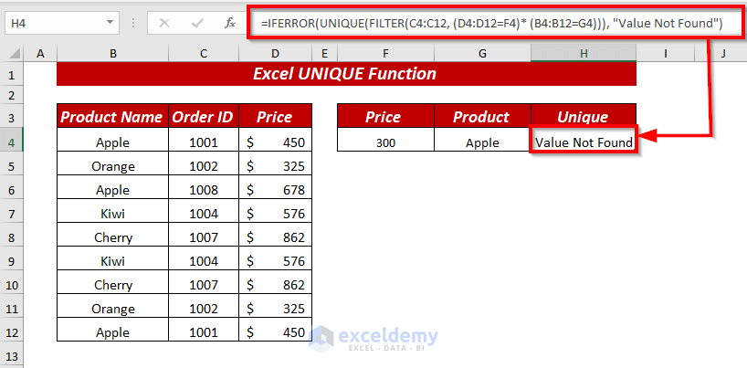
Example 20 – Error Handling with IFERROR
- Scenario: You want to find unique values from a specific range (C4:C12) based on certain conditions (D4:D12 = F4 and B4:B12 = G4). However, if no matching value is found, you want to display Value Not Found instead of an error.
- Formula Explanation:
- UNIQUE(FILTER(C4:C12, (D4:D12=F4) * (B4:B12=G4))): This part of the formula filters the values in the range C4:C12 based on the conditions specified. It returns an array of unique values that meet the criteria.
- IFERROR(UNIQUE(…), “Value Not Found”): The IFERROR function checks if the result of the UNIQUE function contains any errors. If it does, it displays Value Not Found; otherwise, it shows the unique values.
- Step-by-Step Implementation:
- In cell H4, insert the following formula:
=IFERROR(UNIQUE(FILTER(C4:C12, (D4:D12=F4)* (B4:B12=G4))), "Value Not Found")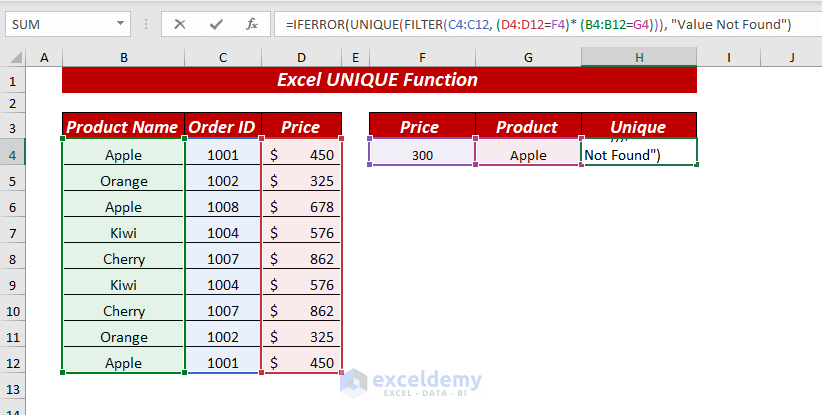
- Press ENTER to calculate the result.
Things to Remember
- #NAME Error: Ensure that you spell the function names correctly (e.g., UNIQUE and FILTER).
- #CALC Error: If no matching value is found, the UNIQUE function will return this error. The IFERROR function handles it by displaying Value Not Found.
- #SPILL Error: If any cells in the spill range are not completely blank, you’ll encounter this error. Make sure the output range (H4 in this case) is empty.
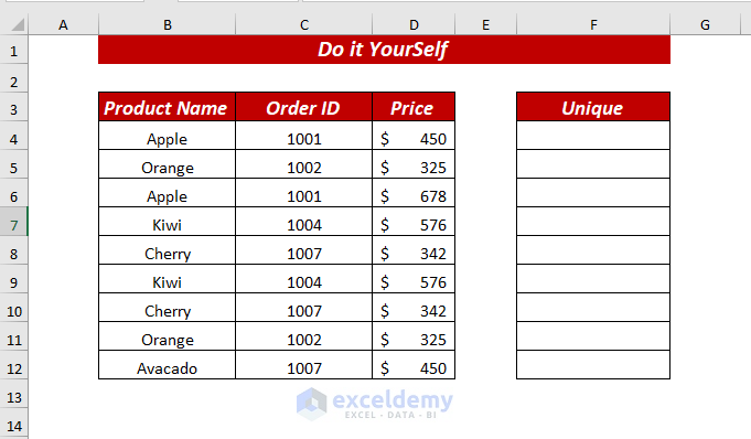
Practice Section
A practice sheet in the workbook to practice these explained examples.
Download to Practice
You can download the practice workbook from here:
<< Go Back to Excel Functions | Learn Excel
Get FREE Advanced Excel Exercises with Solutions!

Hi. Thank you for writing this article. I am having difficulty getting UNIQUE to do what I need, and none of your many examples seems to cover my case.
Even when looking for all unique values within an array, the example data set in this article doesn’t really provide a complete test, because each column is already a different type of information (fruits, numbers, prices). My data has multiple columns of the same type of information, and even when searching for unique values in an array, UNIQUE only evaluates by column or row, listing the unique values within a column or row. So for example, the value “B17” might be present in several columns, and the array returned by UNIQUE will have at least one instance of “B17”, implying that B17 is unique when it is not.
Is there a way to check all cells of an array for uniqueness WITHIN THE WHOLE ARRAY?
Many thanks
Hello Jen,
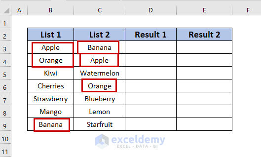
Thanks for your question. I think there is no direct way to fulfill your requirement using the UNIQUE function. But you can use a combination of some functions to get the unique values after comparing different columns.
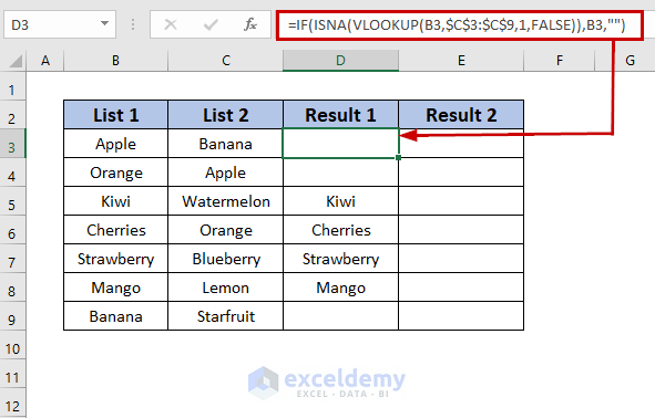
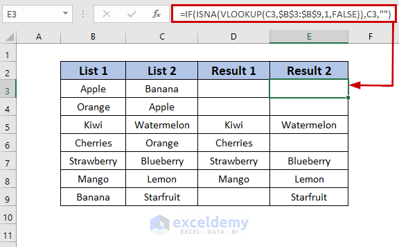
So, I have created the following dataset where I have some names of fruits in the two columns, List 1 and List 2. Here, we have some same fruits names in these two columns, and using the formula we will extract the unique values of these columns in the columns; Result 1, and Result 2.
For extracting the unique values of List 1, we will use the following formula in Result 1.
=IF(ISNA(VLOOKUP(B3,$C$3:$C$9,1,FALSE)),B3,””)
After comparing the unique values of List 2 with the values of List 1 we will use the following formula in the Result 2 column.
=IF(ISNA(VLOOKUP(C3,$B$3:$B$9,1,FALSE)),C3,””)
U have to also show unique values from multiple sheets
Hello, SR! Thanks for your recommendation. We’ll cover this part & give you an update soon.
My query mirrors Jen’s: 20 examples and not one covers database/multiple list style uniqueness queries. Unfortunately, this is common to most sites, which assume people only have interest in business data (Row: a thing, value of the thing, another value of the thing). Sadly, Excel is programmed in the same way. And it extends to help with most functions.
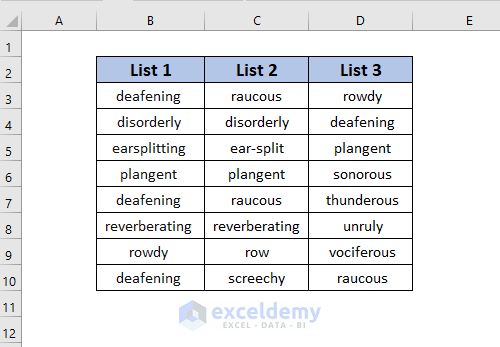
I work with words for most projects to create teaching aids, or qualitative study, and Word doesn’t have formula: my columns are word list A, word list B, C. Row 5 (for example) of my wordlists are unrelated. Reasonably, I want to query unique item. Simply, are any of my words in any list duplicated elsewhere. I wish this was simple. Same with FILTER… I must create this elaborate LET function that knits all the lists together into one column.
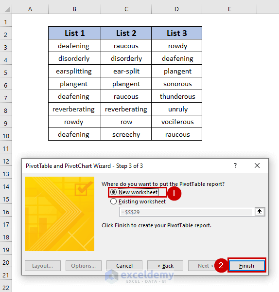
(Example)
Array:
deafening | raucous | rowdy
disorderly | disorderly | deafening
earsplitting | ear-split | plangent
plangent | plangent | sonorous
deafening | raucous | thunderous
reverberating | reverberating | unruly
rowdy | row | vociferous
deafening | screechy | raucous
==|> Array:
deafening | raucous |
disorderly | |
earsplitting | ear-split |
plangent | | sonorous
| | thunderous
reverberating | | unruly
rowdy | row | vociferous
| screechy |
( | = column divide )
All I want, in Jen’s words, is to check unique within a whole array, with simpler formula. And returning words rather than TRUE/FALSE, numbers or errors (when it’s unique), or transformation to a single column.
It’ll be great to see help offered, understanding how to build formula, for any function for people who work with non-related lists (columns) and qualitative data.
Hi Andy,

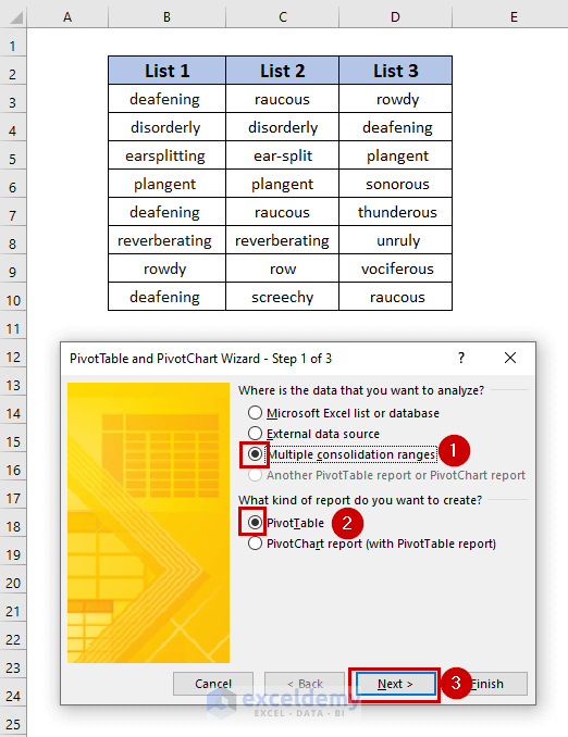

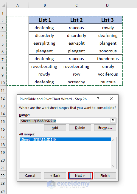
Thanks for your query. Unfortunately, using the UNIQUE function you cannot do your desired job directly. So, I have come up with an easy alternative way.
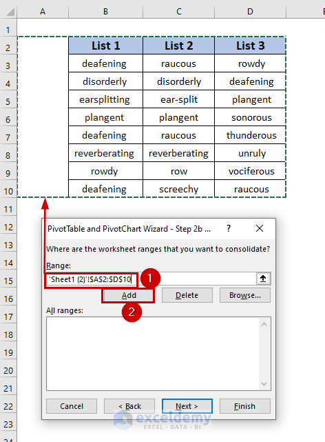
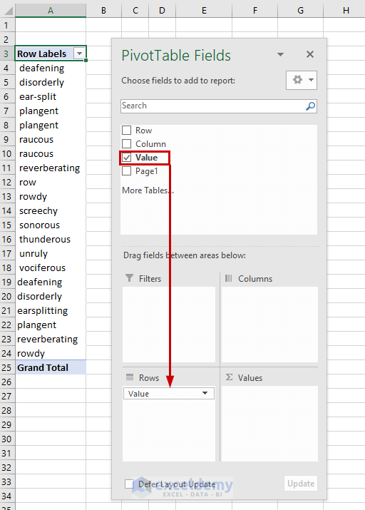
Here, I have created the following dataset using your example. Using the PivotTable feature of Excel, I will convert the following three columns into a single column with unique values only.
• Press ALT+D and then P immediately to open up the PivotTable and PivotChart Wizard.
• In Step 1 of this wizard click on the options; Multiple consolidation ranges, PivotTable.
• Click on Next.
• In Step 2a of this wizard click on the Create a single page field for me option.
• Click on Next.
• Now, select the range of the words including a blank column prior to this range in the Range box.
• Select Add to enter the formula of the Range box to the All ranges box.
Afterward, the formula will be entered into the All ranges box, and finally, click on Next.
• In Step 3 of this wizard click on the New worksheet option.
• Click on Finish.
• Now, drag down the Value to the Rows area.
Finally, all of the unique words will be listed in a single column.