How to Extract Unique Values Based on Criteria in Excel

This is the sample dataset. It showcases the stock of 5 Computer Shops in June and July.

2 Effective Methods to Extract Unique Values Based on Criteria in Excel

Method 1 – Combining the Excel UNIQUE & FILTER Functions to Extract Unique Values

Use the UNIQUE function and the FILTER function.

1.1. Single Criteria

To know which shops have stocked notebooks only , desktops only, or both:

Select E5 and use this formula

=UNIQUE(FILTER(C5:C14,D5:D14=E4))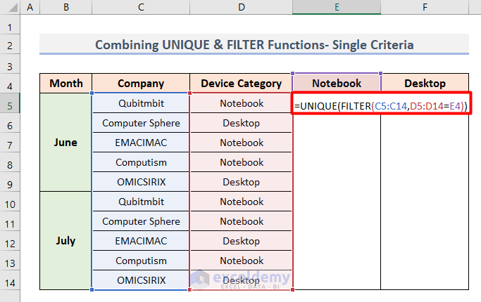

Press Enter and you will see the names of 4 computer shops that have stocked notebooks in the 2 months.

The FILTER function extracts the names of the shops in column C that stocked the notebook in the 2 months. The UNIQUE function shows the names only once.

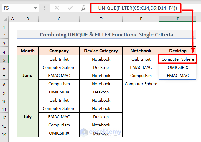
Enter this formula in F5 to find the shop that stocked desktops.

=UNIQUE(FILTER(C5:C14,D5:D14=F4))

Press Enter and you will see the names of 3 shops that stocked desktops in the two months.

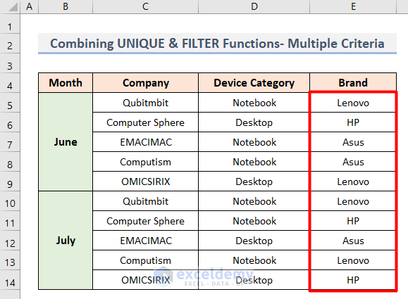
1.2. Multiple Criteria

Find the computer shops that stocked HP notebooks in the 2 months.

Select G12 to display the result.
Enter the formula:

=UNIQUE(FILTER(C5:C14, (D5:D14=D5) * (E5:E14=E6)))

Press Enter.

Only 1 shop stocked HP notebooks in the 2 months.

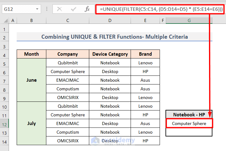
The FILTER function evaluates two criteria- the Device Category and the Brand. The criteria are added using an Asterisk (*). The UNIQUE function shows the shop names only once.

1.3. Multiple Criteria with Alternatives

To find the shops that stocked at least one HP or ASUS device.

Select G11.
Enter this formula.

=UNIQUE(FILTER(C5:C14, (E5:E14=E6) + (E5:E14=E7)))

Press Enter.
You’ll see the names of 4 shops that stocked either HP or ASUS devices .

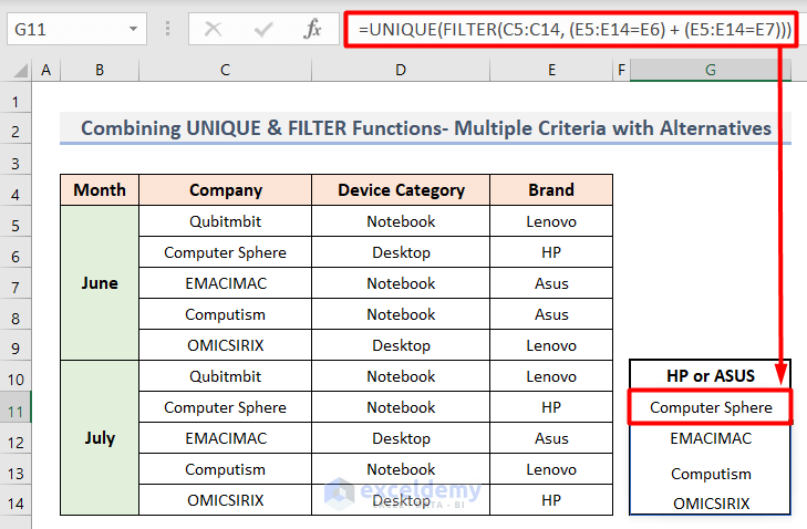
The FILTER function assesses the two criteria separately and shows a combined result. The UNIQUE function shows the names only once.

Method 2 – Using an Array Formula to Extract Unique Values Based on Criteria

2.1. Single Criteria

Find the shops that stocked notebooks or desktops in the 2 months:

In E5, enter this formula.

=IFERROR(INDEX($C$5:$C$14, MATCH(0, IF($E$4=$D$5:$D$14, COUNTIF($E$4:$E4, $C$5:$C$14), ""), 0)),"")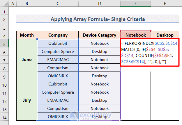

Press Enter.
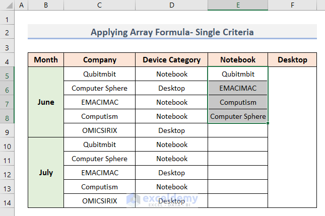
Drag down the Fill Handle to see the result in the rest of the cells.

The names of 4 computer shops are displayed.

In this complex formula,

The COUNTIF function counts the company names and creates an array with a 0 for all company names with multiple occurrences.
The IF function finds the shops that stocked notebooks only and removes 0 from the names of the shops that did not stock notebooks.
The MATCH function searches for 0.
The INDEX function stores all cells in the array as a reference and shows the names of shops with multiple occurrences only once.
The IFERROR function removes error messages and replaces them with empty strings.

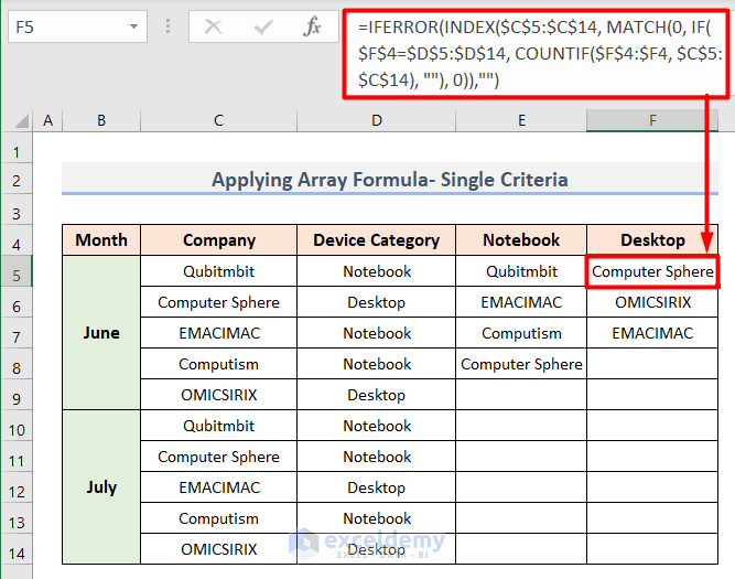
Use the array formula in F5 to find the shops that have Desktop in stock.

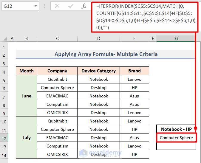
2.2. Multiple Criteria

Find the shops that stocked HP only in the 2 months.

Select G12.
Enter this formula.

=IFERROR(INDEX($C$5:$C$14,MATCH(0,COUNTIF(G$11:$G11,$C$5:$C$14)+IF($D$5:$D$14<>$D$5,1,0)+IF($E$5:$E$14<>$E$6,1,0),0)),"")

Press Enter.
Drag down the Fill Handle to see the result in the rest of the cells.

The IF function is used twice. It first searches for the Notebook category in column D and returns the results as 0 in the array.
It searches for the HP brand in column E and returns the results as 0 in another array.
The COUNTIF function counts the company names and returns the values as 0 in an array for all names found in column C.
The MATCH function searches for the positions of 0 in the 3 arrays.
The INDEX function stores all data as a reference array and shows the names of the shops by row position of the resultant 0.
The IFERROR function removes error messages and displays the shop names only.

How to Extract Unique Values Based on Criteria in Excel – 2 Methods