Method 1 – Using the Excel Array Formula to Extract Unique Items from a List
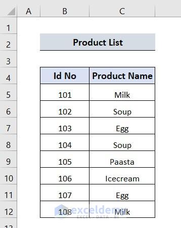
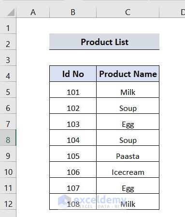
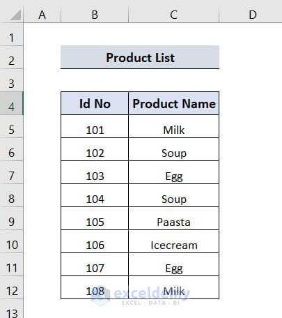
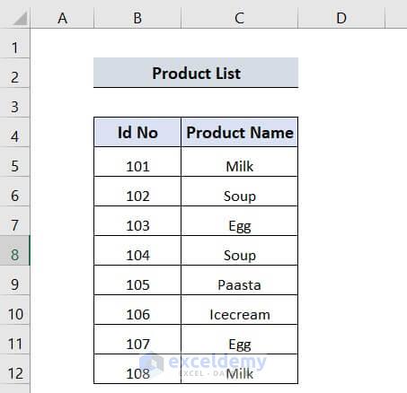
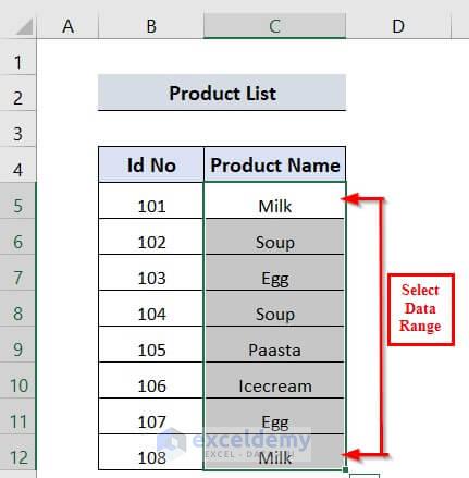
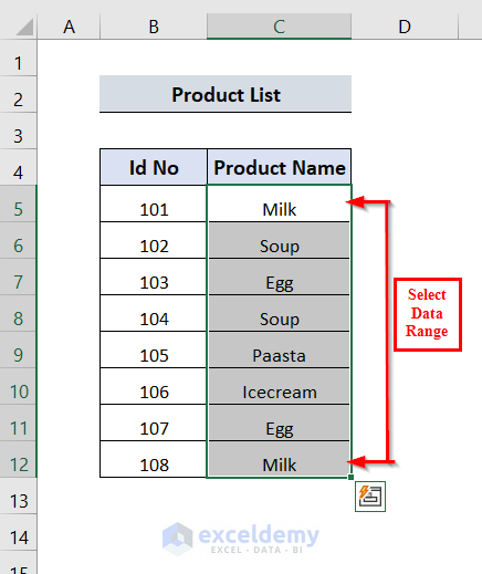
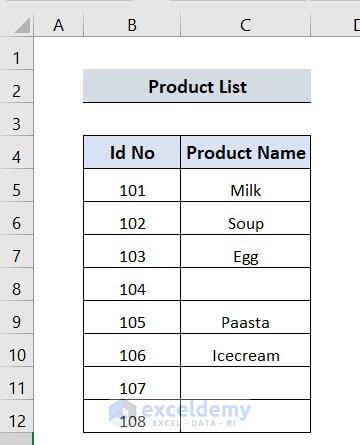
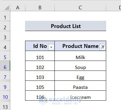
The following Product List contains ID No and Product Name. There is a repetition in Product Name.
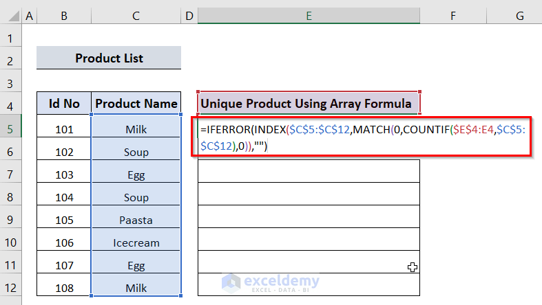
- Enter the following formula in E5.
=IFERROR(INDEX($C$5:$C$12,MATCH(0,COUNTIF($E$4:E4,$C$5:$C$12),0)),"")This formula is a combination of the INDEX, MATCH, and COUNTIF functions.
- COUNTIF($E$4:E4,$C$5:$C$12)→ Checks the unique list and returns 0 when a match is not found and 1 when a match is found.
- MATCH(0,COUNTIF($E$4:E4,$C$5:$C$12),0)→ Identifies the position of the first occurrence of no-match, 0, here.
- INDEX($C$5:$C$12,MATCH(0,COUNTIF($E$4:E4,$C$5:$C$12),0))→ INDEX uses the position returned by MATCH and returns the name from the list.
- The IFERROR function replaces possible errors with blank.
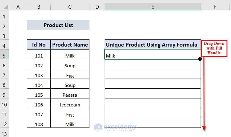
- Press Enter.
- Drag down the formula with the Fill Handle tool.
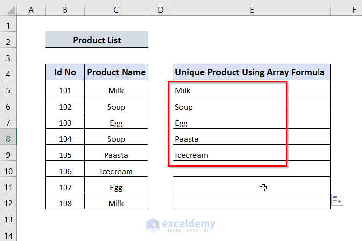
The unique items are displayed in the Unique Products Using Array Formula table.
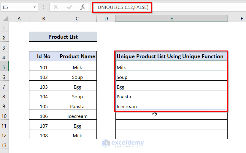
Method 2 – Using the Excel UNIQUE Function to Extract from a List
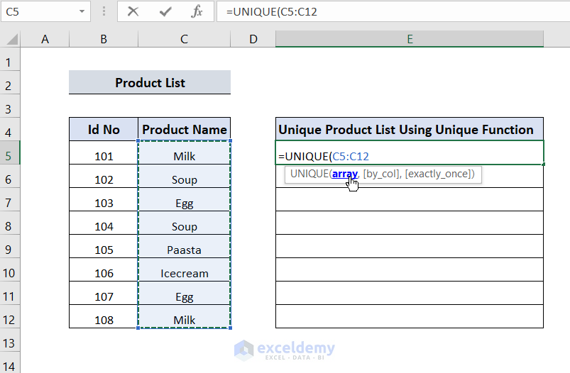
- Enter =UNIQUE in E5 to see the UNIQUE Function.
- Select an array: Product Name, here: C5:C12.
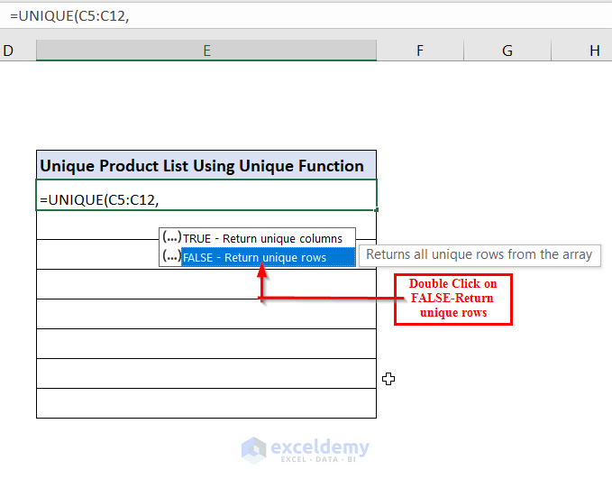
- Enter a comma, ”,”, and double-click False-Return unique rows.
 Close the bracket and press Enter.
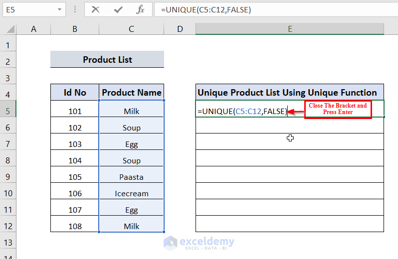
This is the output.
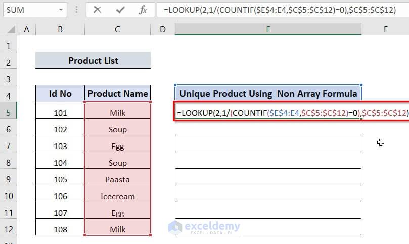
Method 3 – Using the Non-Array Formula with the LOOKUP and COUNTIF Functions
- Enter the following formula in E5.
=LOOKUP(2,1/(COUNTIF($E$4:E4,$C$5:$C$12)=0),$C$5:$C$12)- COUNTIF($E$4:E4,$C$5:$C$12)→ Checks the unique list, and returns a 0 when a match is not found and 1 if a match is found; generates an array of Binary values TRUE and FALSE; divides 1 by this array, providing another array (values 1 and #DIV/0 error).
- The LOOKUP function has 2 as the lookup value. The result of the COUNTIF portion is a lookup_vector. LOOKUP matches the final value of the error and returns the corresponding value.
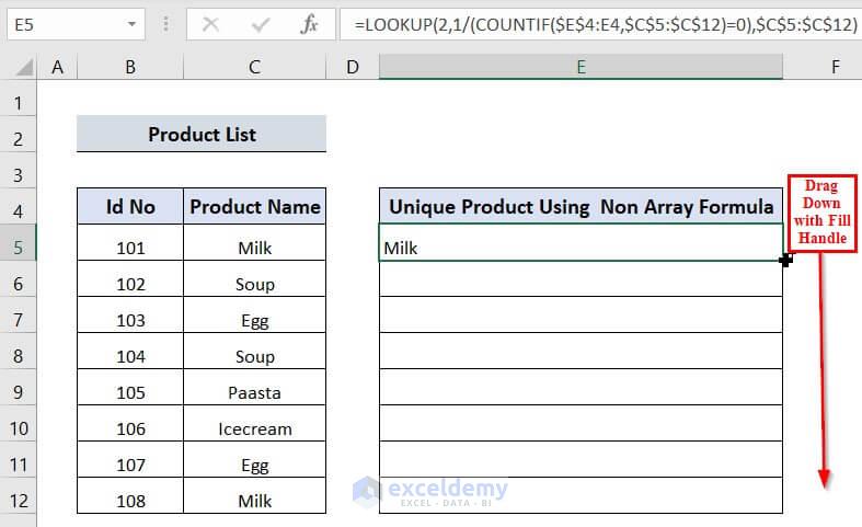
- Press Enter.
- Drag down the formula with the Fill Handle.
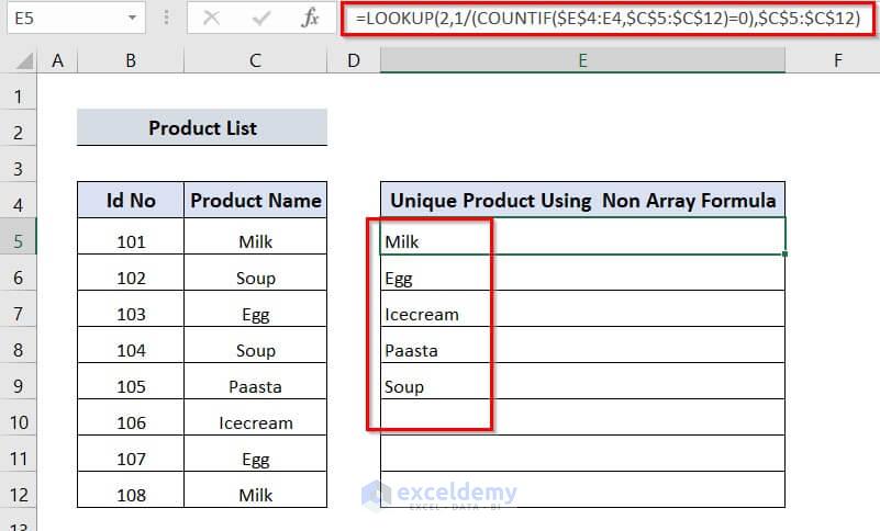
The extracted unique items are displayed in the Unique Product Using Non-Array Formula table.
Method 4 – Extracting Using an Excel Array Formula and
Excluding Duplicates
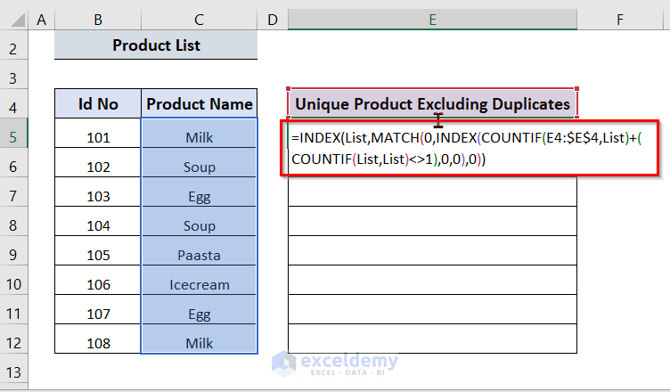
- Enter the following formula in E5.
=INDEX(List,MATCH(0,INDEX(COUNTIF(E4:$E$4,List)+(COUNTIF(List,List)<>1),0,0),0))E4:$E$4 is the first cell of the column we want to exclude and List is the range of selected cells from C5:C12.
The two INDEX functions return the initial and final values returned by COUNTIFS and MATCH.
- Press Enter.
- Drag down the formula with the Fill Handle tool.
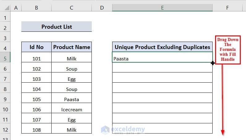
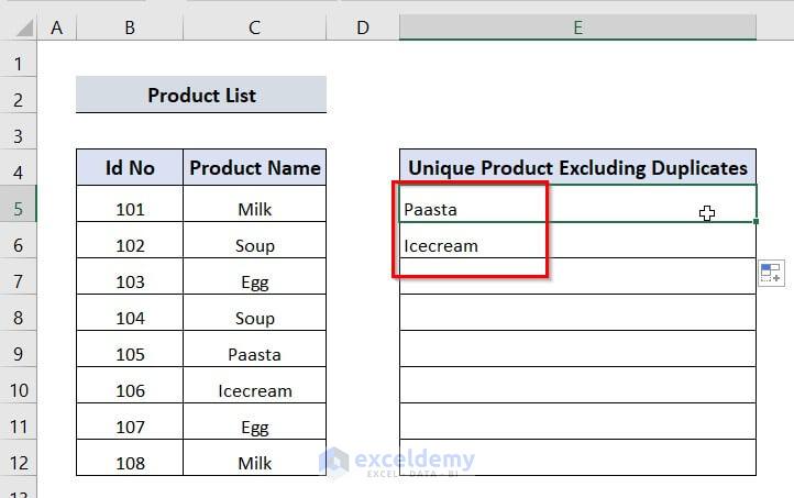
The two unique products are displayed excluding duplications.
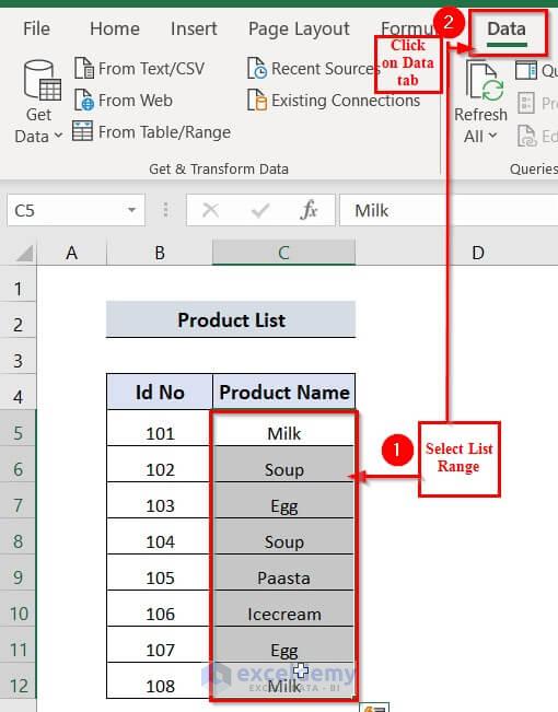
Method 5 – Extracting Unique Items from a List Using an Advanced Filter
- Select the data range.
- Click the Data tab.
- Choose Sort & Filter in Advanced.

- In Advanced Filter, select Copy to another location.
- In Copy to, enter $E$4 .
- Click Unique records only.
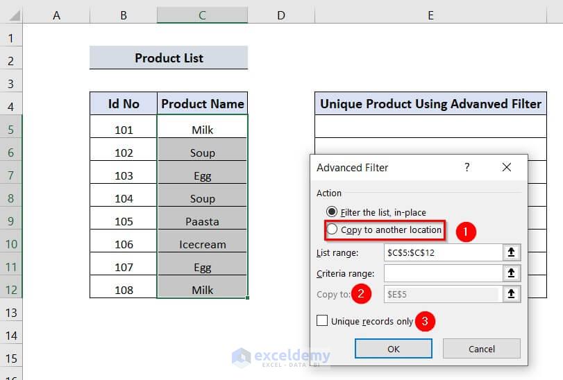
- Click OK.
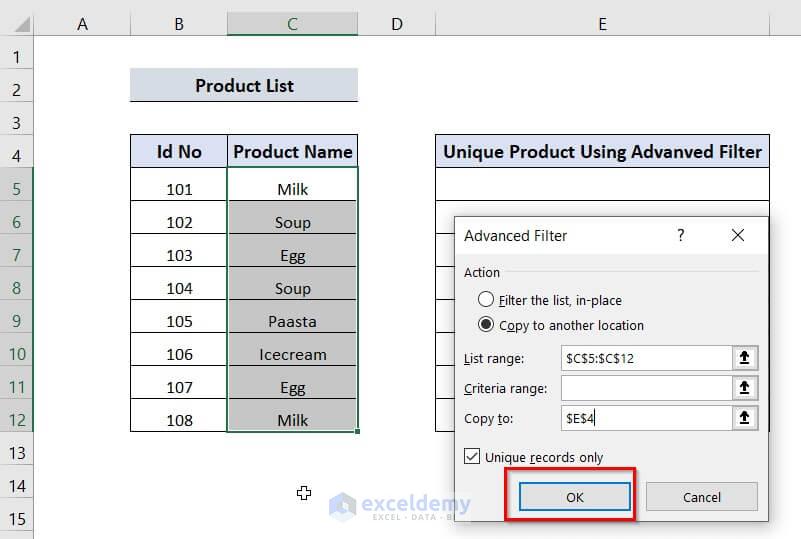
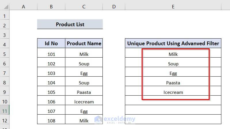
The unique items are extracted in the table Unique Product using Advanced Filter.
Method 6 – Extracting Case-Sensitive Unique Values in Excel
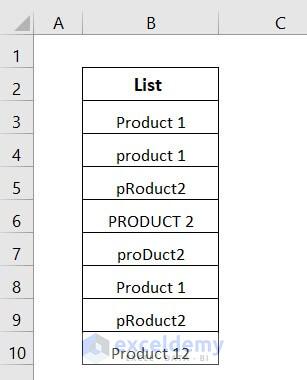
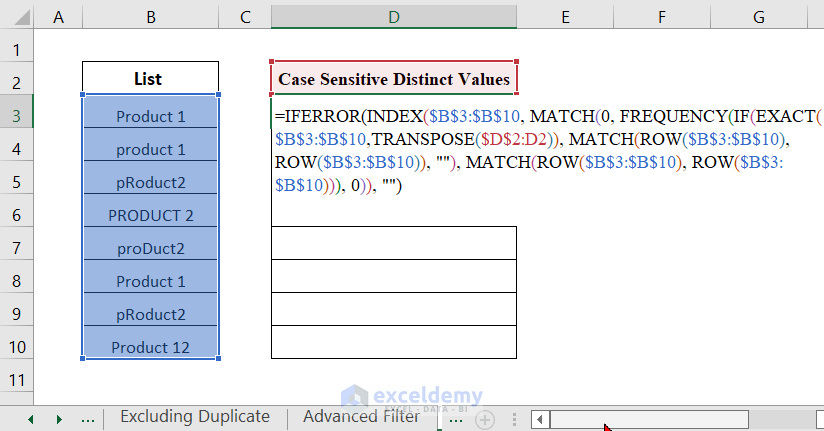
- Enter the following formula in D3.
=IFERROR(INDEX($B$3:$B$10, MATCH(0, FREQUENCY(IF(EXACT($B$3:$B$10,TRANSPOSE($D$2:D2)), MATCH(ROW($B$3:$B$10), ROW($B$3:$B$10)), ""), MATCH(ROW($B$3:$B$10), ROW($B$3:$B$10))), 0)), "")- Press Enter.
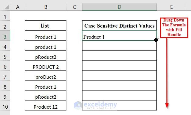
- Drag down the formula with the Fill Handle tool.
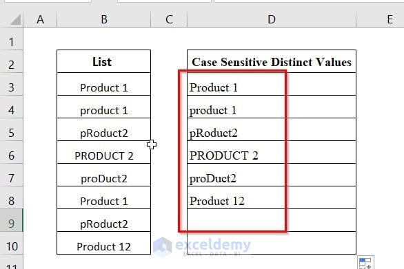
The extracted case-sensitive unique values are displayed in the table Case Sensitive Distinct Values.
Method 7 – Using a Pivot Table to Extract Unique Items from a List

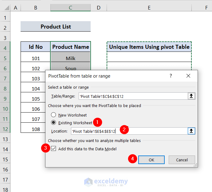
- Select the dataset range. Here, C4:C12.
- Select the Insert tab on the Ribbon.
- Choose Pivot Table.
- Select Existing Worksheet and the location. E4:E12, here.
- Check Add this data to the Data Model.
- Click OK.
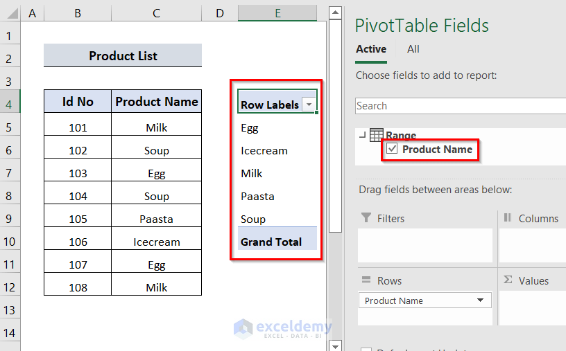
The extracted Unique Product is displayed in the Row Levels table.
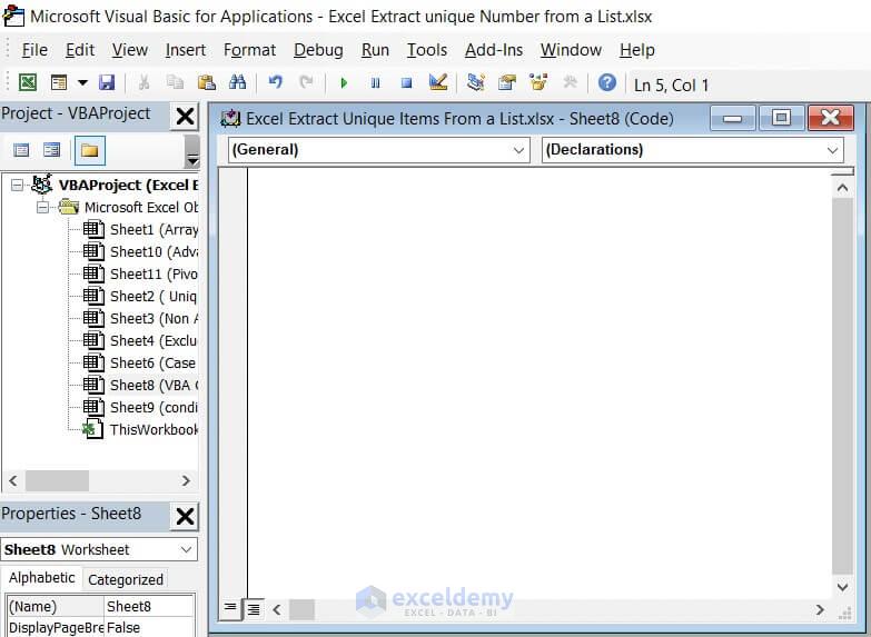
Method 8 – Applying a VBA Macro to Extract Unique Items from a List
- Press ALT+F11 in the active sheet. Here, Sheet8.
- A VBA window will appear.
- Double-click Sheet8.
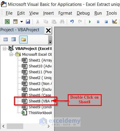
The VBA editor is displayed.
- Enter the following code.
Sub ExtractUnique()
Rem Declare a Long type variable
Dim lsrow As Long
Rem Define the variable
lsrow = Cells(Rows.Count, "C").End(xlUp).Row
Rem Applying AdvancedFilter
ActiveSheet.Range("C4:C" & lsrow).AdvancedFilter Action:=xlFilterCopy, _
CopyToRange:=ActiveSheet.Range("E4"), Unique:=True
End Sub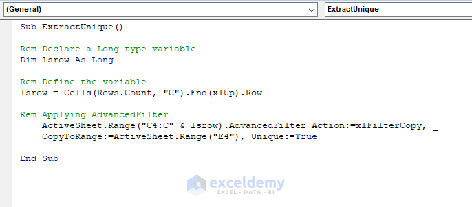
- Close the VBA editor and go to Sheet8.
- Press ALT+F8 to open the Macro.
- Click Run.
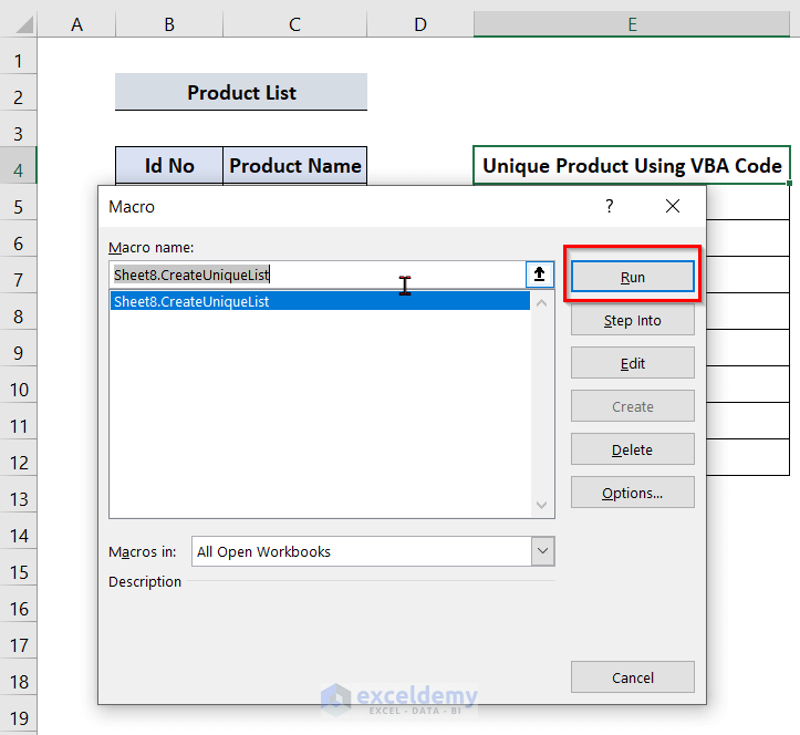
The unique products are displayed in the Product Name table.
Method 9. Highlighting Unique Items with Conditional Formatting
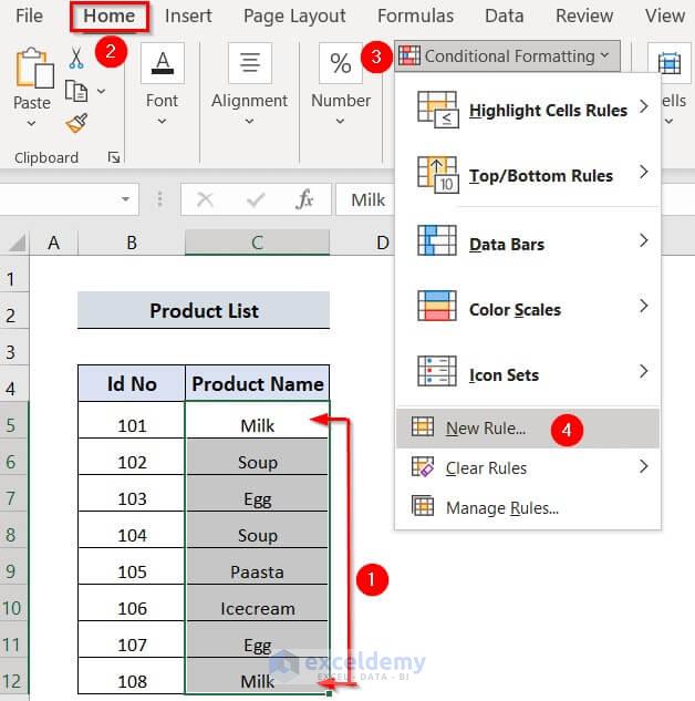
- Select the Product Name (C5:C12).
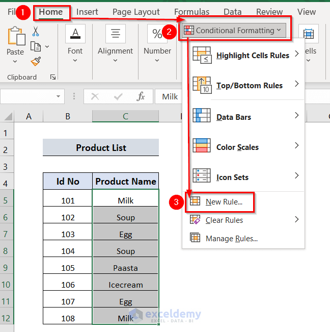
- Go to the Home tab.
- Select Conditional Formatting.
- Choose New Rule.
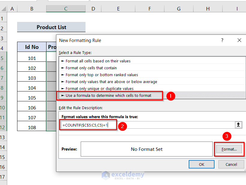
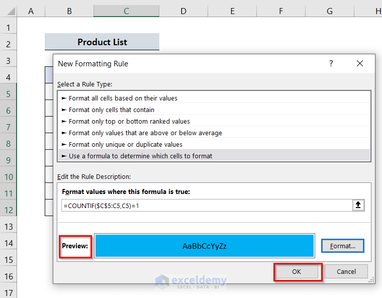
- In the New Formatting Rule window, select Use a Formula to determine which cells to format.
- Enter the following formula in Format values where this formula is true.
=COUNTIF($C$5:C5,C5)=1- Click Format.
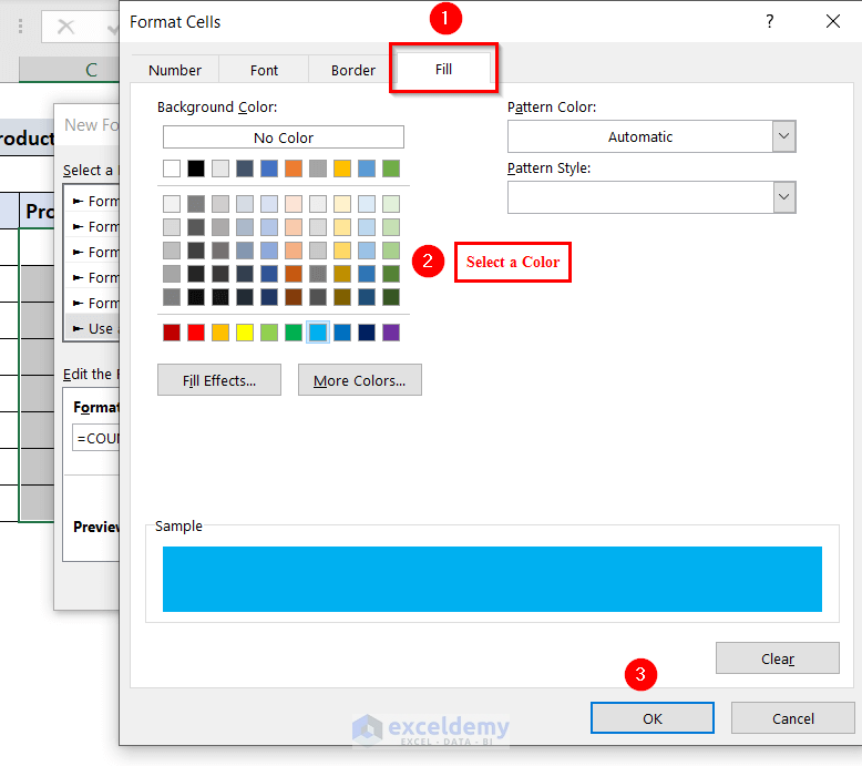
- In Format Cells: click Fill.
- Select a color. Blue, here.
- Click OK.
- Preview and click OK.
The highlighted unique Product Name is displayed.

Method 10. Using Conditional Formatting to Extract Unique Items
- Select the Product Name (C5:C12).
- Go to the Home tab on the Ribbon and select Conditional Formatting.
- Choose New Rule.
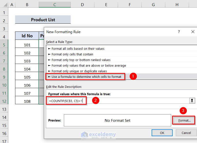
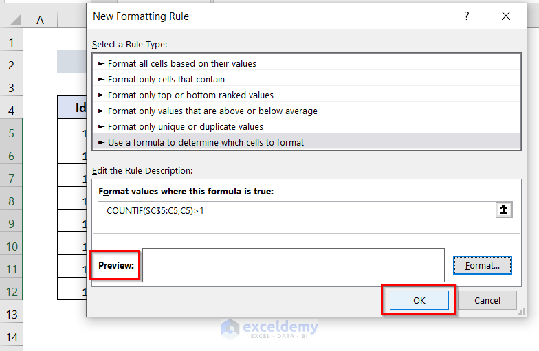
- In New Formatting Rule, select Use a Formula to determine which cells to format.
- Enter the following formula in Format values where this formula is true.
=COUNTIF($C$5:C5,C5)>1- Click Format.
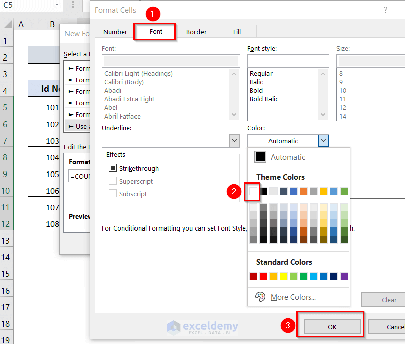
- In Format Cells, select Font.
- Select a white Theme Color.
- Click OK.
- Preview and click OK.
The duplicate product names are hidden (colored white).
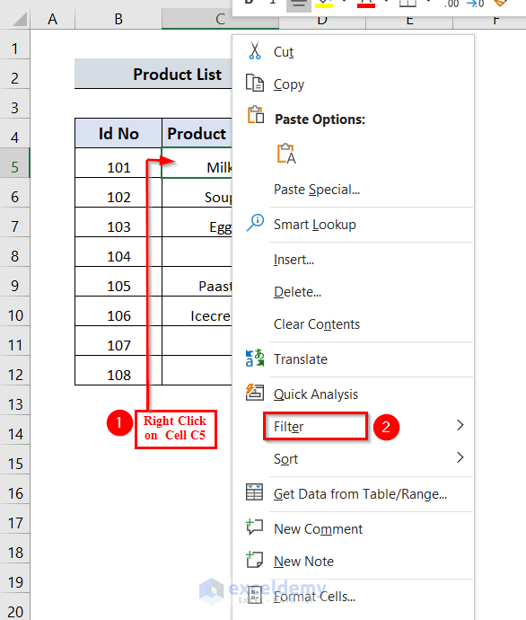
- Right-click any cell to sort unique products Here, C5.
- Select Filter.
- Choose Filter by Selected Cells Font Color.
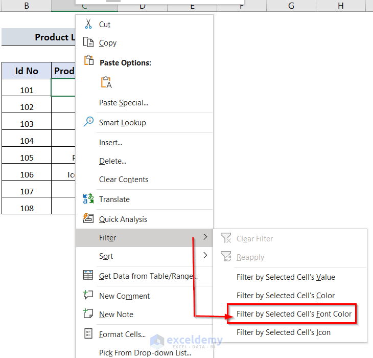
The unique Product Name is displayed in the Product List table.
Download Workbook
<< Go Back to Learn Excel
Get FREE Advanced Excel Exercises with Solutions!
