How to Find Unique Values from Multiple Columns in Excel (5 Easy Ways)

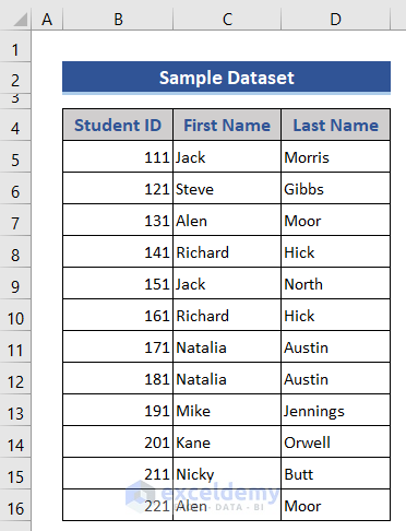
We have a record of student IDs and names. We want to extract the unique values.

Method 1 – Extract Unique Values from Multiple Columns with Array Formula

Case 1 – Using the UNIQUE Function

We want to extract the unique values from both the First Names (Column C) and the Last Names(Column D).

• Select a result cell and insert the following formula there.

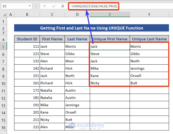
• We have got the Unique Names in two different columns.

We have inserted by_col as FALSE, so it did not search along the columns We have also inserted exactly_once as TRUE, so it did return the values that appear only once.

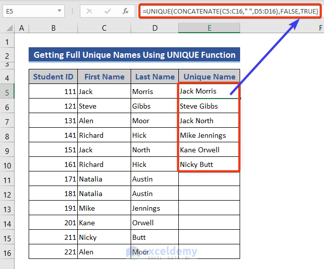
Case 2 – Combining CONCATENATE and UNIQUE Functions

Let’s get a complete list of full names.

First Formula:

Alternative Formula:

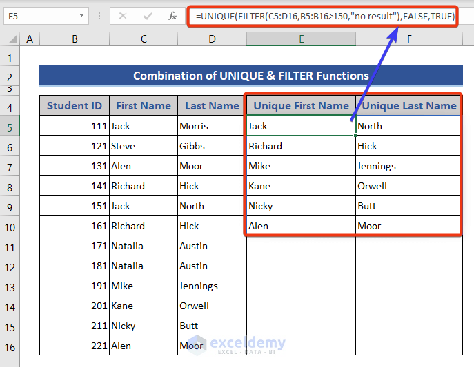
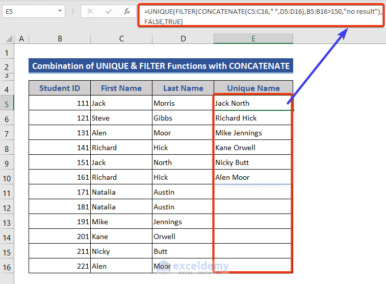
Case 3 – Using UNIQUE, CONCATENATE, and FILTER Functions to Extract Unique Values Based on Criteria

Let’s extract the unique names of the students whose IDs are greater than 150.

• Use the following formula:

• If you want to extract the full unique names in one cell, use this formula:

Method 2 – Highlight Duplicate Values Using Conditional Formatting

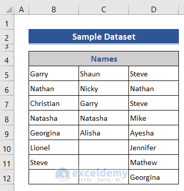
We have three columns, but all with the same type of data. We’ll highlight the duplicates.

Steps:

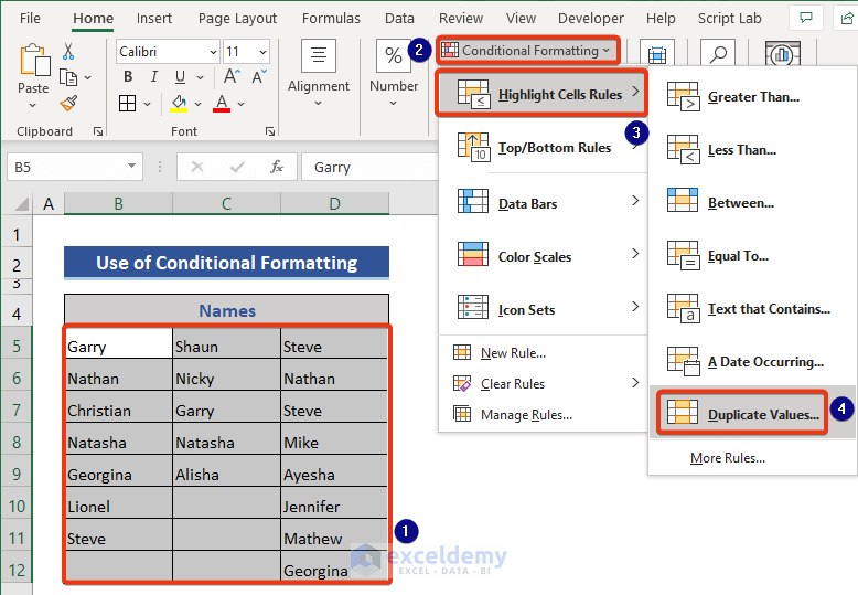
• Select the dataset.
• Go to Home and select Conditional Formatting, then choose Highlight Cells Rules and select Duplicate Values.

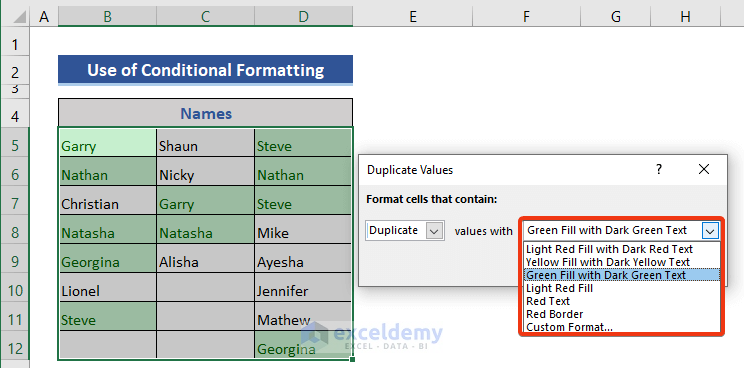
• You will get a small box called Duplicate Values.
• Select any color in the second box to highlight the duplicate values.
• Click OK.

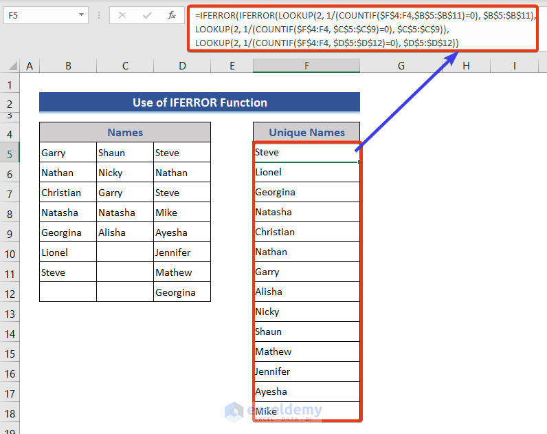
Method 3 – Extract Unique Values from an Excel Column Using a Non-Array Formula

Steps:

• Select any cell.
• Insert the following formula-

• Drag the Fill Handle and you will find the unique names.

Method 4 – Extract a Unique Distinct List from Two or More Columns Using a Pivot Table

Steps:

• Press Alt + D. then press P. You will get the PivotTable and PivotChart Wizard opened.
• Select Multiple consolidation ranges and PivotTable.

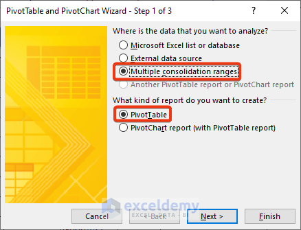
• Click Next. You will move to Step 2a of 3.
• Select Create a single page field for me.

• Click Next. You will go to Step 2b.
• In the Range box, select the range of your cells with an empty column on the left. We have selected cells B5 to D12.
• Click Add. Your selected cells will be added to the All ranges box.

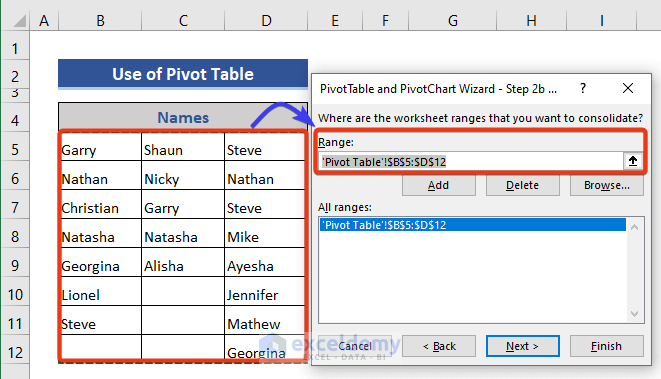
• Click Next. You will move to Step 3.
• In the Existing worksheet box, select the cell where you want the Pivot Table. We put $F$4.

• Click Finish. You will get a Pivot Table.
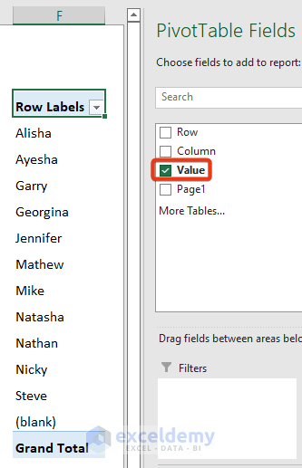
• In the Choose fields to add to report part, unmark Row, Column, Value, Page 1.

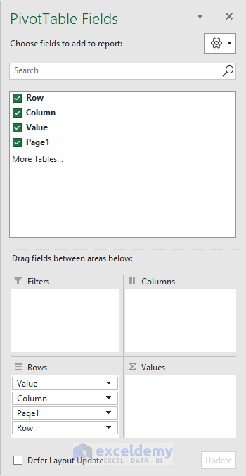
• Select Value. You will get the unique names in the Pivot Table.

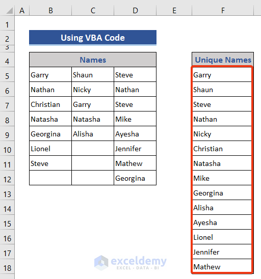
Method 5 – Use VBA Code to Find Unique Values

Steps:

• Press Alt + F11 on your workbook to open the VBA window.
• Go to the Insert tab in the VBA toolbar and choose Module.

• You will a get new Module window.
• Insert the following code:

Sub Uniquedata()
Dim rng As Range
Dim InputRng As Range, OutRng As Range
Set dt = CreateObject("Scripting.Dictionary")
xTitleId = "Select Range"
Set InputRng = Application.Selection
Set InputRng = Application.InputBox("Range :", xTitleId, InputRng.Address, Type:=8)
Set OutRng = Application.InputBox("Output to (single cell):", xTitleId, Type:=8)
For Each rng In InputRng
    If rng.Value <> "" Then
        dt(rng.Value) = ""
    End If
Next
OutRng.Range("A1").Resize(dt.Count) = Application.WorksheetFunction.Transpose(dt.Keys)
End Sub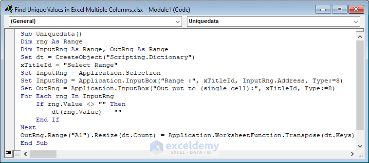

• Save the file as an Excel Macros Enabled Workbook.
• Go back to the workbook.
• Press Alt + F8.
• You will get the Macro box.
• Select the name of the Macro and then click on Run. The name of this Macro is Uniquedata.
• Enter the range of your data in the Range box.

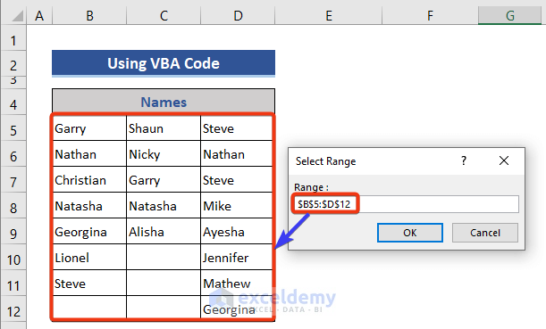
• Click on OK. You will get another input box.
• Enter the first cell where you want the unique names. We put cell F5.

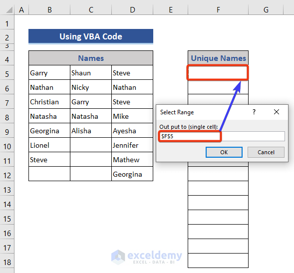
• Cclick OK. You will get unique names from your data set.

Download the Practice Workbook

<< Go Back to Learn Excel