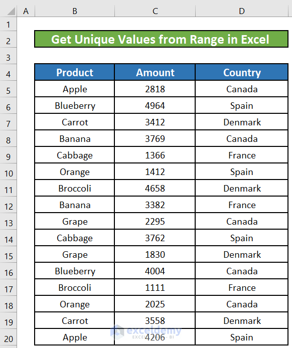
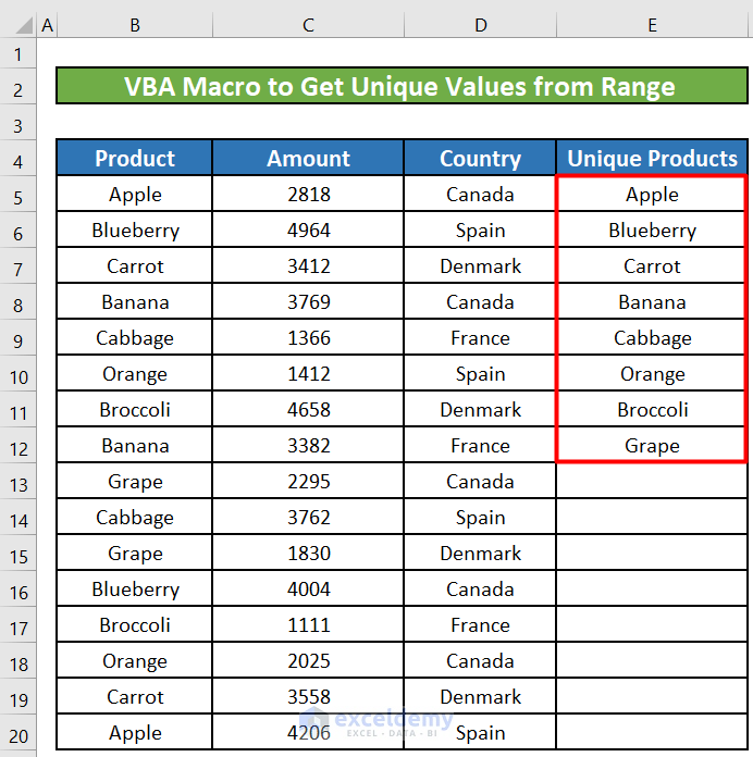
Let’s assume a scenario where we have an Excel file that contains information about the products that a country exports to different countries in Europe. We have the Product name, exported Amount, and the Country to which the product is exported. We will find every unique product that this country exports and each distinct country that this country exports the product to.
Method 1 – Use Advanced Filter to Get Unique Values From a Range
Steps:
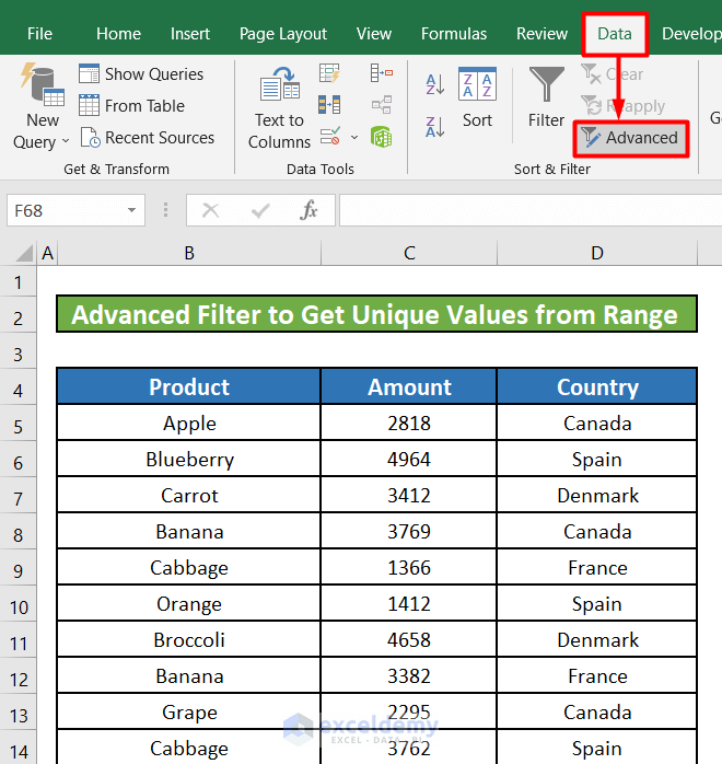
- Go to the Data tab.
- Select Advanced from the Sort & Filter section.
- A new window titled Advanced Filter will appear. Choose Copy to another location as Action.
- In the List Range box, select the range you want to extract the unique values from. In this example, we are trying to get all the unique or distinct products under our Product column (B5:B20). So, our List Range will be $B$5:$B$20. $ signs have been inserted to make the cell references absolute.
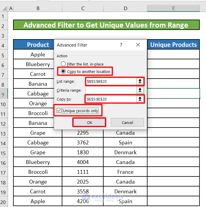
- In the Copy to box, select a range where the unique values will be. We have selected the range E5:E20. Check the box with the title Unique records only.
- Click OK.
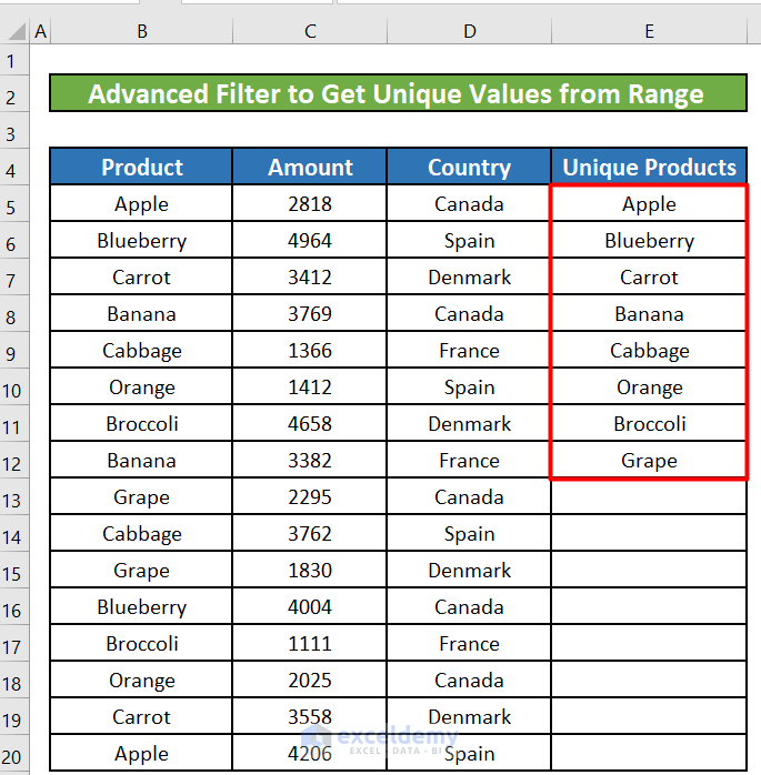
- You will get all the distinct products in the Unique Products column (E5:E20).
Method 2 – Insert the INDEX and MATCH Formula to Get Unique Values From Range
Steps:
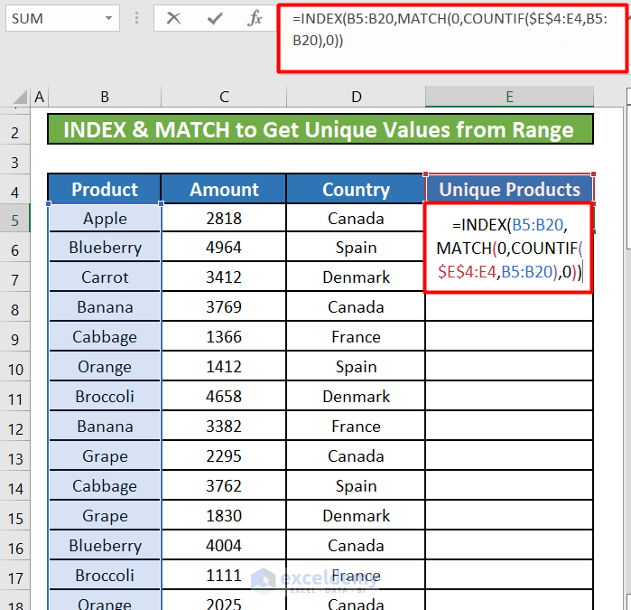
- Select cell E5. Use this formula in the cell:
=INDEX(B5:B20,MATCH(0,COUNTIF($E$4:E4,B5:B20),0))The driving force of this formula is the INDEX function which will perform the basic lookup.
=INDEX(array, row_num, [column_num])
INDEX function has two required arguments: array and row_num.
So, if we provide the INDEX function with an array or list as the first argument and a row number as the second argument, it will return a value that will be added to the unique list.
We have provided B5:B20 as the first argument. But the hard part is to figure out what we will give the INDEX function as the second argument or row_num. We have to choose the row_num carefully so that we will only get unique values.
We will achieve this using the COUNTIF function.
=COUNTIF($E$4:E4,B5:B20)
The COUNTIF function will count how many times items in the Unique Product column appear in the Product column which is our source list.
It will use an expanding reference. In this case, it is $E$4:E4. On one side, an expanding reference is absolute, while on the other, it is relative. In this scenario, the reference will extend to include more rows in the unique list as the formula is copied down.
Now that we have the arrays, we can start looking for row numbers. To find zero values, we use the MATCH function, which is set up for the precise match. If we use MATCH to combine the arrays generated by COUNTIF, the MATCH function locates the items while searching for a count of zero. When there are duplicates, MATCH always returns the first match. So, it will work.
Finally, INDEX provides the positions as row numbers, and INDEX returns the name at these positions.
- You will get the value Apple in cell E5.
- Drag the fill handle downward to apply the formula to the rest of the cells.
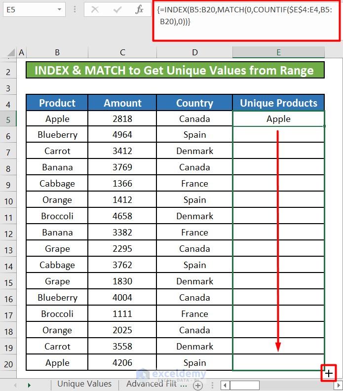
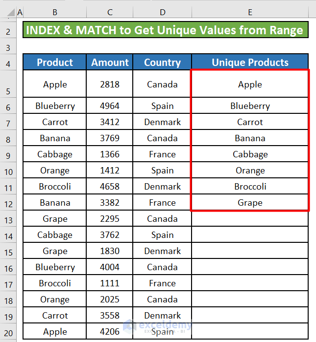
- We will get all the unique values in the Unique Products.
Method 3 – Apply the INDEX and MATCH Formula to Get Unique Values with Empty Cells
We have removed some of the products from the range.
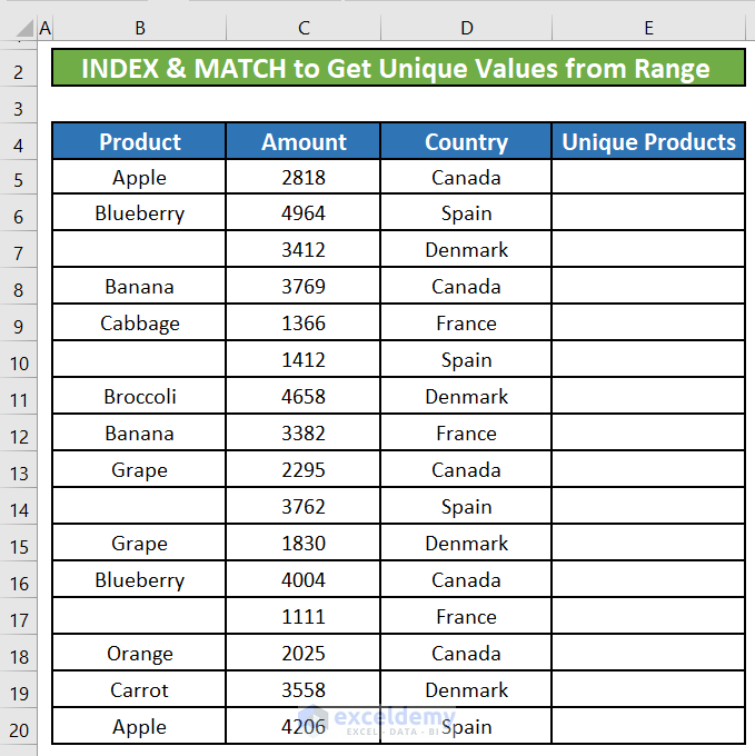
Steps:
- Use the following formula in Cell E5.
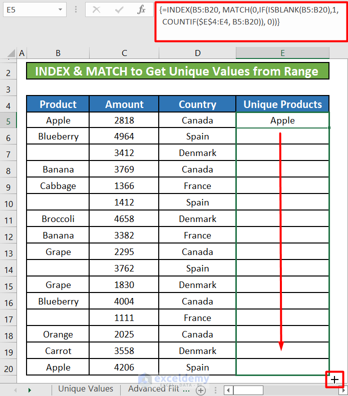
=INDEX(B5:B20, MATCH(0,IF(ISBLANK(B5:B20),1,COUNTIF($E$4:E4, B5:B20)), 0))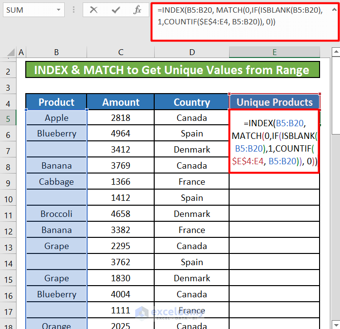
- You will get the value Apple in cell E5.
- Drag the fill handle down to apply the formula to the rest of the cells.
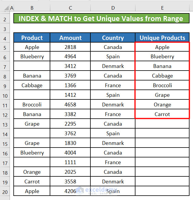
- We will get all the unique values in the Unique Products.
Method 4 – Use the LOOKUP and COUNTIF Formula to Get Unique Values From a Range
Steps:
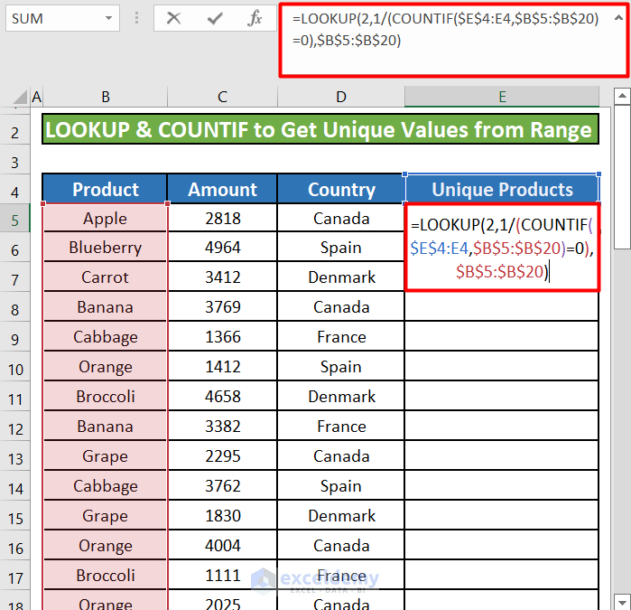
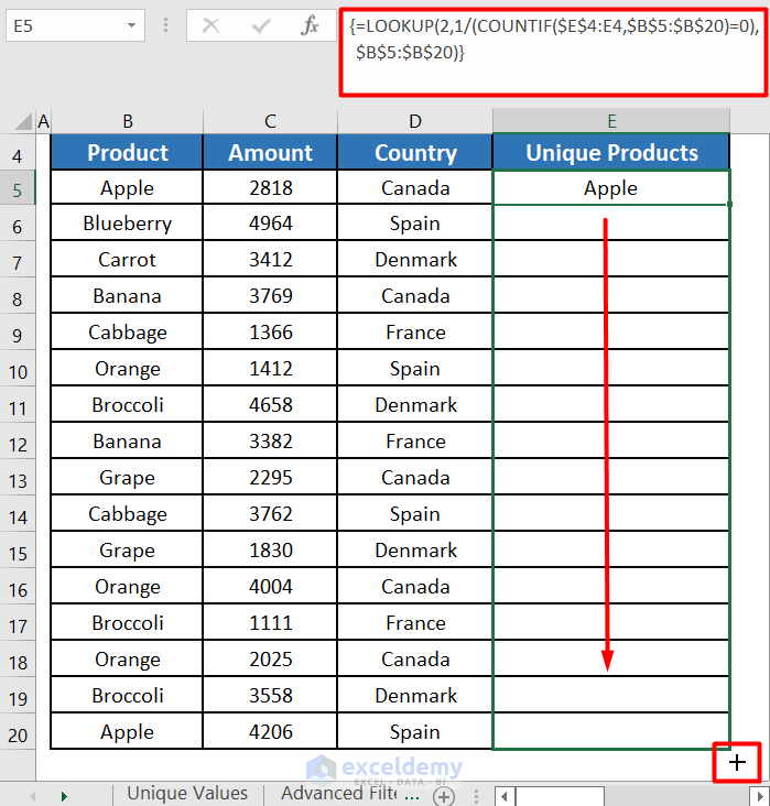
- Select cell E5. Insert the following formula in it:
=LOOKUP(2,1/(COUNTIF($E$4:E4,$B$5:$B$20)=0),$B$5:$B$20)The structure of the formula is similar to that of the combination of the INDEX and MATCH formula above, but LOOKUP handles array operations natively. The LOOKUP function takes three arguments exactly.
=LOOKUP(lookup_value, lookup_vector, [result_vector])
COUNTIF produces a count of each value in the expanding range $E$4:E4 from the range $B$5:$B$20. Then the count of each value is compared to zero and an array consisting of TRUE and FALSE values is generated.
Then the number 1 is divided by the array, resulting in an array of 1s and #DIV/0 errors. This array becomes the second argument or the lookup_vector for the LOOKUP function.
The lookup_value or the first argument of the LOOKUP function is 2 which is greater than any of the lookup vector’s values. The last non-error value in the lookup array will be matched by the LOOKUP.
LOOKUP returns the corresponding value in result_vector or the third argument for the function. In this case, the third argument or the result_vector is $B$5:$B$20.
- You will get the value Apple in cell E5.
- Drag the fill handle down to apply the formula to the rest of the cells.
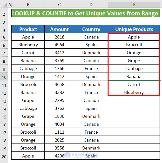
- We will get all the unique values in the Unique Products.
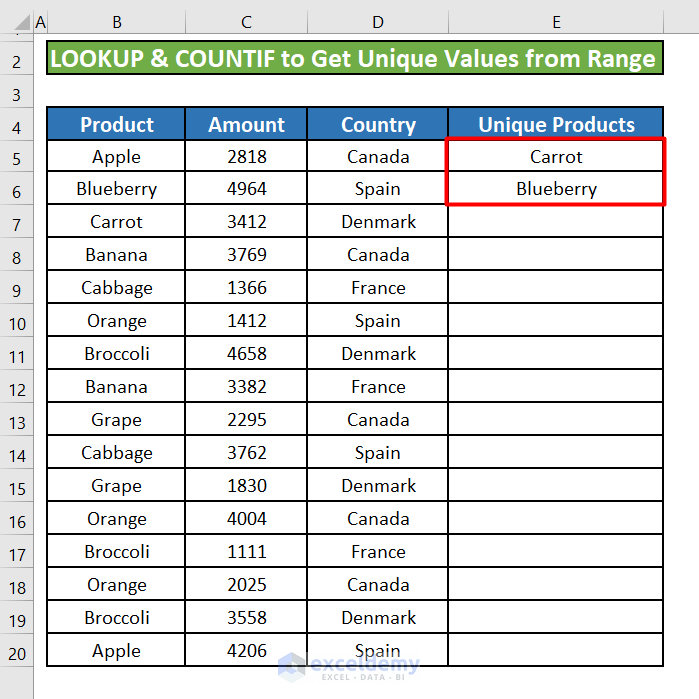
Method 5 – Use the LOOKUP and COUNTIF Formula to Get Unique Values that Appear Only Once
We have modified our Excel worksheet so that we the products Blueberry and Carrot appear only once in our worksheet. We will get these two unique values that appear only once in our worksheet.
Steps:
- Select cell E5 and insert the following formula:
=LOOKUP(2,1/((COUNTIF($E$4:E4,$B$5:$B$20)=0)*(COUNTIF($B$5:$B$20,$B$5:$B$20)=1)),$B$5:$B$20) 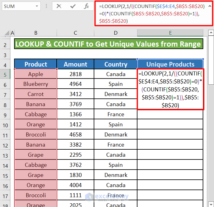
- You will get the value Carrot in cell E5.
- Drag the fill handle down to apply the formula to the rest of the cells.
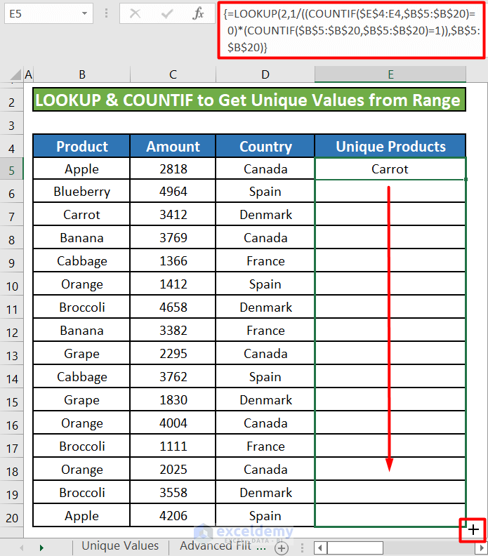
- We will get the 2 unique values that appear once only in cells E5 and E6 under the Unique Product. The rest of the cells below them will show the #N/A value.
Method 6 – Use the UNIQUE Function to Get Unique Values in the Range
Microsoft Excel 365 has a function called UNIQUE that returns a list of unique values in a specific range.
Steps:
- Select cell E5. Use the following formula in the cell.
=UNIQUE(D5:D20) 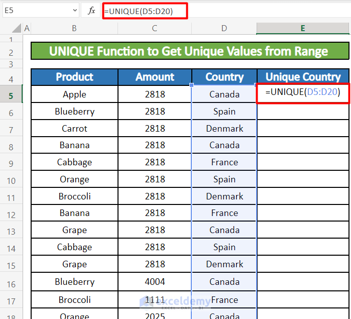
- If we press Enter, we will get all the unique countries in our Unique Country column.

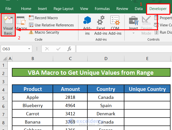
Method 7 – Run a VBA Macro Code in Excel to Get Unique Values in the Range
Steps:
- Select Visual Basic from the Developer or press Alt + F11 to open a VBA window.
- Click on the Insert button and select Module.
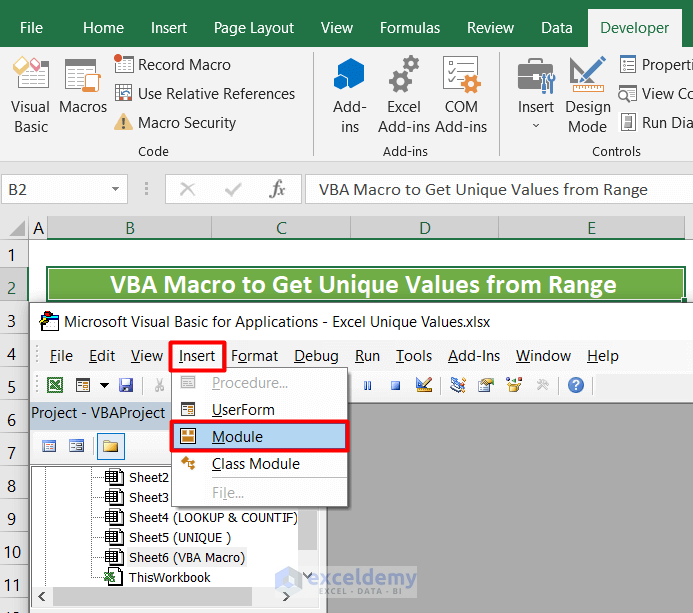
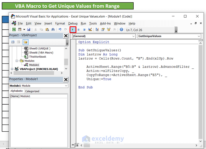
- Insert the following code in the module:
Option Explicit
 Sub GetUniqueValues()
Dim lastrow As Long
lastrow = Cells(Rows.Count, "B").End(xlUp).Row
       ActiveSheet.Range("B5:B" & lastrow).AdvancedFilter _
    Action:=xlFilterCopy, _
    CopyToRange:=ActiveSheet.Range("E5"), _
    Unique:=True
End Sub- Click on the Run button to execute the code.
- We will get all the unique products in the Unique Products column.
Method 8 – Remove Duplicates in Excel to Get Unique Values in the Range
Steps:
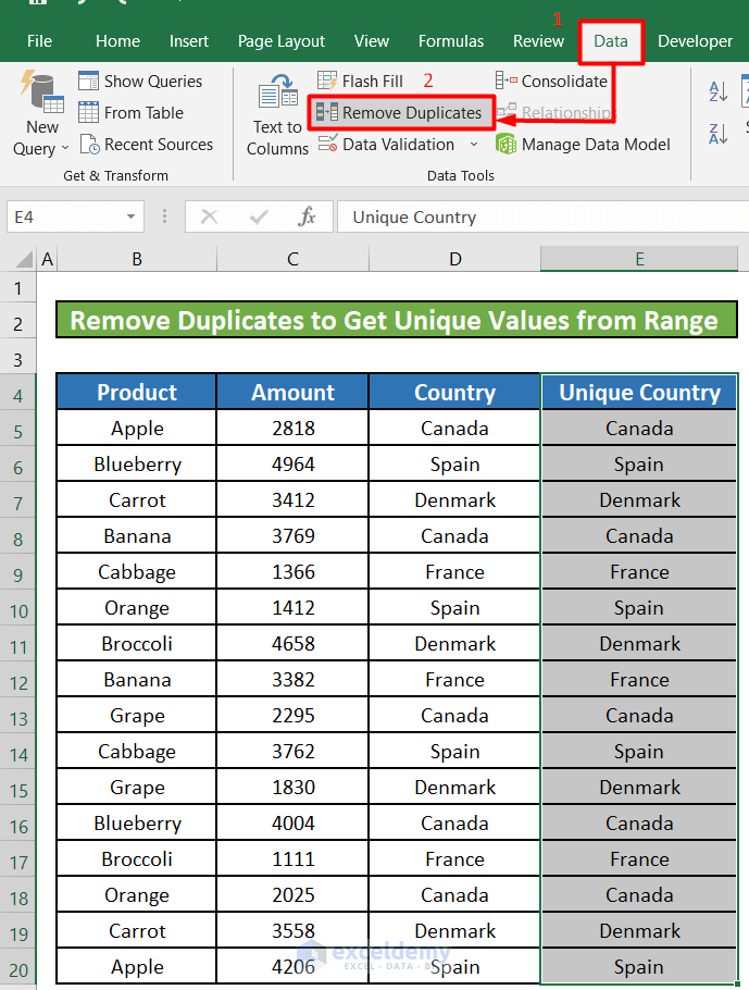
- Select all the cells under Country.
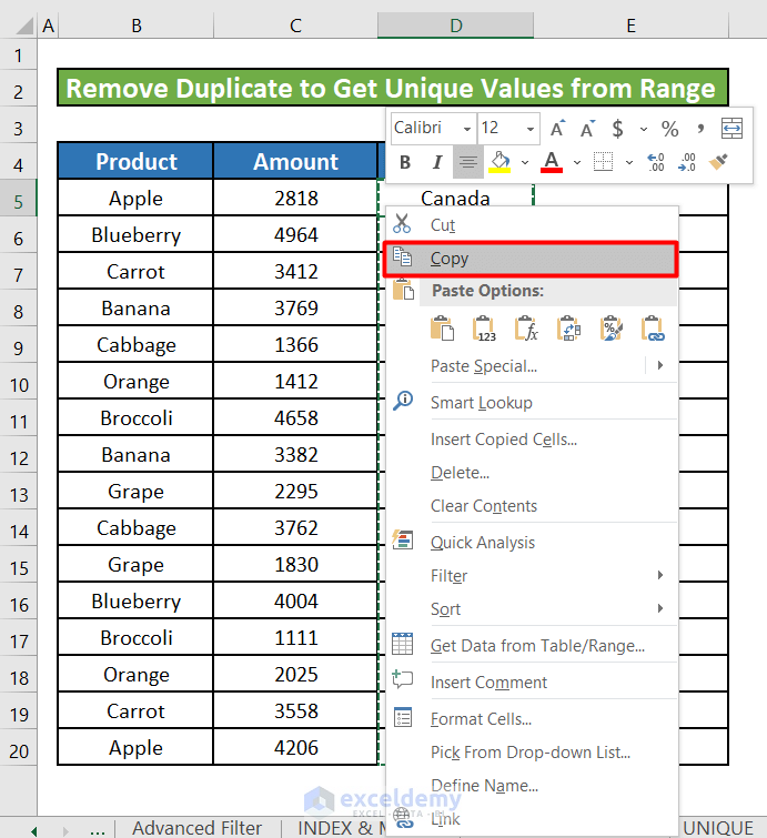
- Paste the range in the adjacent Unique Country. Select the new column.
- Select the Remove Duplicates option from the Data tab.
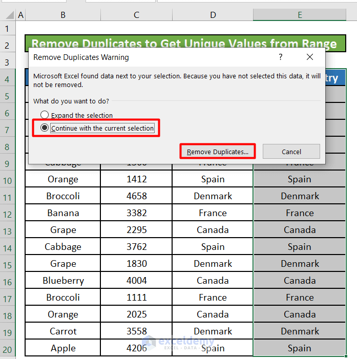
- A new window titled Remove Duplicates Warning will appear. Select Continue With Current Selection.
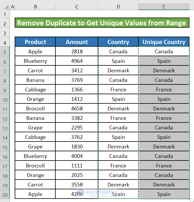
- Click on Remove Duplicates.
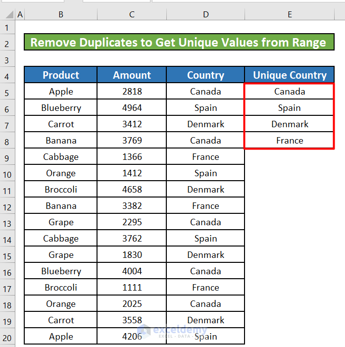
- We will see our Unique Country column has only 4 unique countries in it.
Things to Remember
- The INDEX and MATCH functions together are an array formula. So, you must press CTRL+SHIFT+ENTER together to insert the formula in a cell. It will put two curly braces around the whole formula.
- While using the Remove Duplicates feature to get unique values from the range, we have selected only the Unique Country But you can add more columns or select all the columns by selecting the Expand the selection option. But if you expand the selection to add more columns, then the Remove Duplicates feature will not remove any value unless it finds two or more rows with identical data.
Download the Practice Workbook
<< Go Back to Learn Excel
Get FREE Advanced Excel Exercises with Solutions!

thank you!
Hello April,
You are most welcome. Thanks for your appreciation.
Keep exploring Excel with ExcelDemy!
Regards,
ExcelDemy