How to Build Lightweight Machine Learning Models in Excel Using Solver and Formulas

 

Excel is a surprisingly powerful tool for basic machine learning tasks.  Though it’s not a machine learning platform, it can be effectively used to demonstrate foundational ML concepts like linear and logistic regression using built-in functions and Solver.

In this tutorial, we will show how to build lightweight machine learning models in Excel using Solver and formulas.

• Linear Regression: Predict continuous values (sales revenue, house prices, test scores, etc.).
• Logistic Regression: Predict yes/no outcomes (customer purchases, loan defaults, medical diagnosis, pass/fail, etc.).

Prerequisites:

• Microsoft Excel (2016 or later recommended).
• Enable Solver Add-in.
  • Go to the File tab >> select Options >> select Add-ins >> select Excel Add-ins.
  • Click Go.

• • Select Solver Add-in.
  • Click OK.

• Basic understanding of regression concepts.

Part 1: Linear Regression Model

Linear regression finds the best straight line to predict continuous numerical values through the data points. We will model a simple business scenario where advertising spend (X) predicts sales revenue (Y). Each data point represents one month of business data.

Step 1: Setting Up Sample Data

Create a realistic dataset that shows a clear linear relationship between input (advertising spend in thousands) and output (sales revenue in thousands).

Each row is one month of business data. As advertising spend increases, sales revenue increases too, but not perfectly (there’s some randomness, which is realistic).

Step 2: Create Prediction Formula

Set up the mathematical “knobs” that our model will adjust to find the best line. In linear regression, we need two parameters:

• Intercept (b0): Where the line crosses the Y-axis (baseline sales with $0 advertising).
• Slope (b1): How much sales increase for each $1000 increase in advertising.

Set up the model parameters in separate cells:

Model Parameters:

Predicted Y = b0 + b1 * X

• Intercept (b0)
• Initial value 0
• Slope (b1)
• Initial value 1

We will use this linear equation to predict sales based on advertising spend. This is the core of the model, and it takes the advertising amount and estimates what sales should be.

Mathematical Meaning:

• If b0 = 0.5 and b1 = 2, then spending $3k on advertising predicts: 0.5 + 2*3 = $6.5k in sales.
• The model learns the best values for b0 and b1 from the data.

Prediction Formula:

• Select a cell and insert the following formula.

=$E$3 + $E$5 * A2

• Drag this formula down to F11.

Step 4: Calculate Residuals and Errors

Measure how wrong our predictions are. This is crucial because the model learns by trying to minimize these errors.

• Residuals: The difference between actual sales and predicted sales for each month.
• Squared Errors: Residuals squared (to make all errors positive and penalize large errors more).

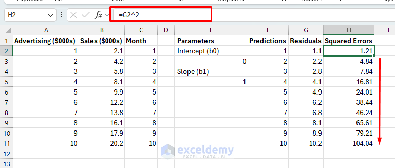
Residuals:

=B2 - F2

• Drag down the formula to G11.

Squared Errors:

=G2^2

• Drag down the formula to H11.

Step 5: Calculate Error Metrics

Create business-meaningful measurements of model performance. These metrics help to understand if the model is good enough for real-world use.

Set up key metrics in a designated area:

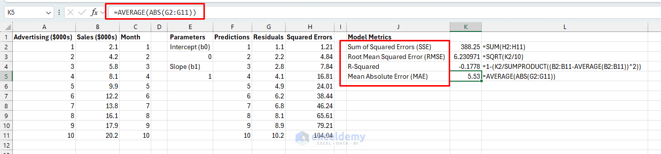
Error Metrics:

• Sum of Squared Errors (SSE): Total error across all predictions – lower is better.

=SUM(H2:H11)

• Root Mean Squared Error (RMSE): Average error in original units ($000s) – easier to interpret.

=SQRT(K2/10)

• R-Squared: Percent of sales variation explained by advertising (0-100%, higher is better).

=1-(K2/SUMPRODUCT((B2:B11-AVERAGE(B2:B11))^2))

• Mean Absolute Error (MAE): Average absolute error – less sensitive to outliers than RMSE.

=AVERAGE(ABS(G2:G11))

Step 6: Use Solver to Optimize Parameters

Let Excel automatically find the best values for intercept and slope that minimize prediction errors.

• Go to the Data tab >> select Solver.
• Set Objective: K2 (SSE cell).
• To: Min.
• By Changing Variable Cells: E3,E5 (your parameters).
• Click Solve.

• Click OK.

• It tries millions of different combinations of b0 and b1.
• Calculates the total error for each combination.
• Keeps adjusting until it finds the combination with the lowest error.
• This is much faster and more accurate than guessing.

Step 7: Create Visualization

Visual validation of the model makes sense. Let’s see the prediction line passing close to most data points.

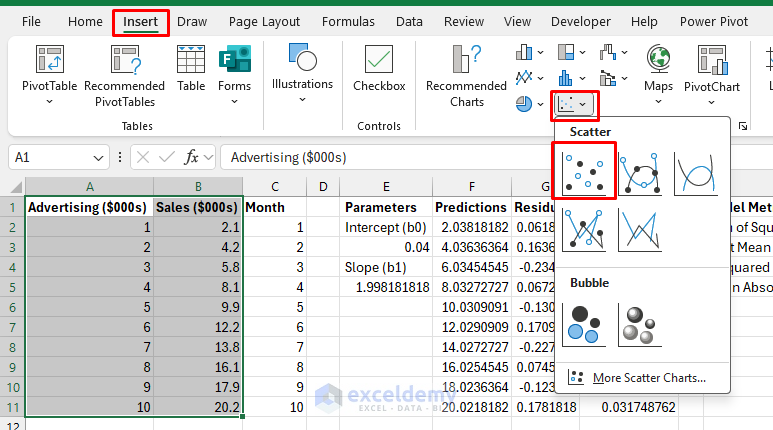
• Select the Advertising and Sales columns.
• Go to the Insert tab >> from Charts >> select Scatter Plot.

• Right-click the chart >> select Data >> select Add Series.
  • Series Name: Select cell F1.
  • Series X Values: Select X-values (e.g., B2:B11)
  • Series Y Values: Click and select the predicted values F2:F11.
• Format the prediction series as a line.

• The prediction line follows the general trend of the data points.
• Points are scattered around the line (not all above or below).
• No obvious patterns in the residuals.

Part 2: Logistic Regression Model

Logistic regression predicts probabilities for yes/no decisions. Unlike linear regression, which predicts exact numbers, logistic regression predicts the likelihood of something happening (0-100%).

Step 1: Prepare Binary Classification Data

Let’s model customer purchase behavior. Based on customer income level (X), we want to predict whether they’ll buy our premium product (1) or not (0). This is typical for marketing targeting, medical diagnosis, or any binary decision.

Set up data for logistic regression:

Customer income levels (in $10k units) and purchase decisions. Notice how lower-income customers (1-5) tend not to buy (0), while higher-income customers (6-10) tend to buy (1). This reflects realistic purchasing patterns.

Step 2: Create Logistic Prediction Formula

Initialize Logistic Model Parameters:

Set up parameters for the logistic function. Unlike linear regression, these parameters work through a more complex mathematical transformation (the sigmoid function).

• Intercept (b0): Shifts the threshold left or right (where 50% probability occurs).
• Slope (b1): Controls how steep the transition is from “unlikely” to “likely”.
• Starting Values: We start with reasonable guesses; the Solver will optimize them.

Logistic Parameters:

Probability = 1 / (1 + e^(-(b0 + b1×X)))

• Intercept (b0)
• -2 (Initial value)
• Slope (b1)
• 0.5 (Initial value)

Create Logistic Prediction Formula:

Transform linear combinations into probabilities using the sigmoid function. This is the mathematical magic that keeps predictions between 0 and 1.

• Linear Combination: b0 + b1*X (same as linear regression).
• Sigmoid Transform: 1/(1+e^(-(linear combination))) converts any number to the 0-1 range.
• Result: A smooth S-curve that represents probability. If the probability is 0.7, there’s a 70% chance this customer will buy.

Probability Predictions: 

• Linear Combination:

=$E$3 + $E$5 * A2

• Probability Predictions:

=1/(1+EXP(-F2))

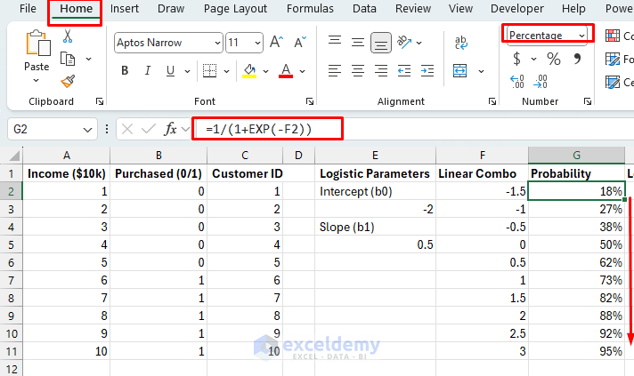
• Format the cells as Percentage (%).

Step 4: Calculate Log-Likelihood

Measure how well our probability predictions match the actual outcomes. This is more complex than simple errors because we’re dealing with probabilities, not exact values.

Log-Likelihood Components:

=IF(B2=1,LN(MAX(G2,0.0001)),LN(MAX(1-G2,0.0001)))

• For binary outcomes, we can’t use simple subtraction (actual – predicted).
• Instead, we measure how “surprised” we are by the actual outcome given our prediction.
• If we predict a 90% chance of purchase and the customer buys, we’re not surprised (good model).
• If we predict a 10% chance of purchase and the customer buys, we’re very surprised (bad model).

Step 5: Set Up Logistic Model Metrics

Create business-relevant measures of classification performance. These metrics helps to decide if the model is good enough for making real business decisions.

High precision means fewer wasted marketing dollars (low false positives). High recall means we don’t miss potential customers (low false negatives).

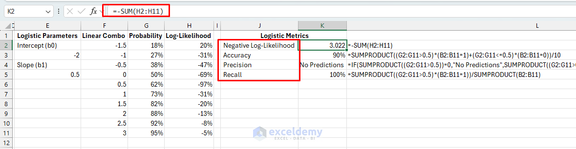
Logistic Metrics:

• Model Fit/Negative Log-Likelihood: Lower values mean better probability predictions.

=-SUM(H2:H11)

• Accuracy: Percent of customers correctly classified (if we use 50% as a cutoff).

=SUMPRODUCT((G2:G11>0.5)*(B2:B11=1)+(G2:G11<=0.5)*(B2:B11=0))/10

• Precision: What percent of the customers we predicted would buy, and what percent bought?

=IF(SUMPRODUCT((G2:G11>0.5))=0,"No Predictions",SUMPRODUCT((G2:G11>0.5)*(B2:B11=1))/SUMPRODUCT((G2:G11>0.5)))

• Recall: What percent of the customers who bought, what percent did we identify?

=SUMPRODUCT((G2:G11>0.5)*(B2:B11=1))/SUMPRODUCT(B2:B11)

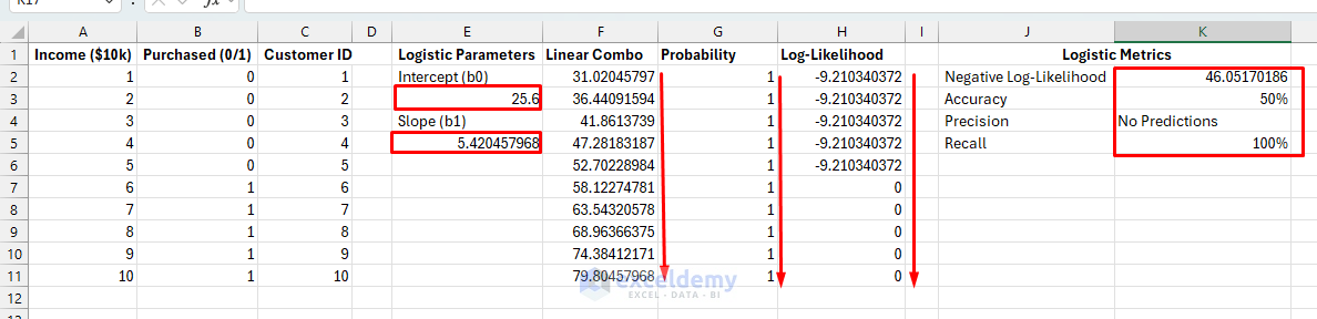
Step 6: Optimize the Logistic Model with Solver

Find the parameter values that best fit the probability pattern in the data. Solver minimizes the negative log-likelihood, which maximizes the probability of observing the actual data.

• Go to the Data tab >> select Solver.
• Set Objective: K2 (Negative Log-Likelihood).
• To: Min.
• By Changing Variable Cells: E3,E5.
• Click Solve.

Troubleshoot Common Issues

• Solver not converging: Try different initial values or increase iterations.
• Negative R-squared: Check for data entry errors or model specification.
• Perfect separation in logistic: Reduce feature values or add regularization.

Conclusion

This tutorial shows the step-by-step procedure to build a machine learning model directly in Excel. While Excel has limitations compared to specialized ML tools, it offers transparency and accessibility for understanding model mechanics. By using Excel’s Solver and basic formulas, you can quickly implement these lightweight machine learning models, visualize predictions, and understand model accuracy through a simple yet insightful method. The techniques shown here can be extended to more complex scenarios and serve as educational tools for learning regression concepts.