An Overview of the SORT Function in Excel:
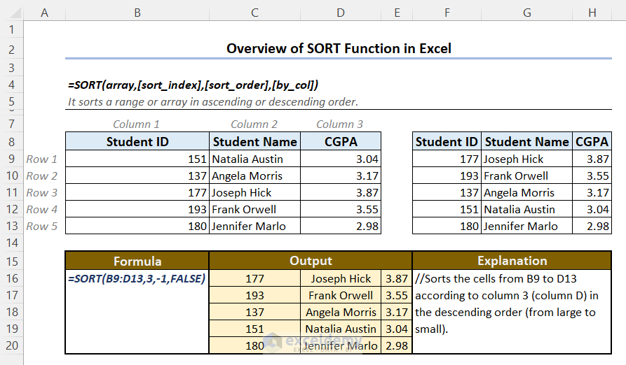
Introduction to the SORT Function in Excel: Syntax and Arguments
⦿ Objective:
Sorts a given range of cells according to a specific row or column in ascending or descending order.
⦿ Syntax:
The syntax of the SORT function is:
=SORT(array,[sort_index],[sort_order],[by_col])
⦿ Arguments:
| Argument | Type | Value |
|---|---|---|
| array | Required | The range of cells that is to be sorted. |
| [sort_index] | Optional | The number of the specific row or column according to which you want to sort the table. The default is 1. |
| [sort_order] | Optional | An integer denotes whether to be sorted in ascending order or descending order. -1 for descending order, 1 for ascending order. Default is 1 (Ascending order) |
| [by_col] | Optional | A boolean value (TRUE or FALSE) indicates whether to be sorted through rows or columns. The default is FALSE. |
Notes:
[sort_index] is the number of the row or column according to which you want to sort the whole table. It must be a number. If it is a fraction, Excel will convert it to an integer, but will raise #VALUE! error if it is not a number.
⦿ Return Value:
Returns a table of cells sorted according to a specific row or column.
⦿ Available in:
Excel for Microsoft 365 | Excel for Microsoft 365 for Mac | Excel for the web | Excel 2021 | Excel 2021 for Mac | Excel for iPad | Excel for iPhone | Excel for Android tablets | Excel for Android
How to Use the SORT Function in Excel: 4 Suitable Examples
- We have sorted the table according to column 3 (CGPA) in descending order. The applied formula is:
=SORT(B5:D9,3,-1,FALSE)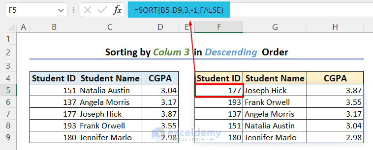
[sort_order] denotes whether to be sorted in ascending order or descending order. -1 for descending order, 1 for ascending order. It must be either -1 or 1 or fractions that become -1 or when 1 is converted to integers, like 1.3 or -1.7, etc. If it is not, Excel will raise #VALUE! error.
- We have sorted the table according to column 1 (Student ID) in ascending order. The formula we have used is:
=SORT(B14:D18,1,1,FALSE)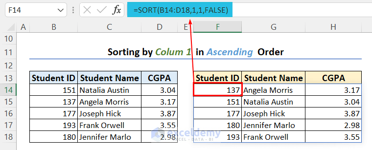
[by_col] is a Boolean value (the default is FALSE.) indicating whether to be sorted through rows or columns. You can use numbers in place of Boolean values. In that case, only 0 will denote FALSE, all other numbers will denote TRUE. That means, by default, the table is sorted through rows. But if you set it as TRUE, the table will be sorted through columns.
- We have sorted the table in ascending order through the columns, according to row number 3. The formula used here is:
=SORT(B23:D27,3,1,TRUE)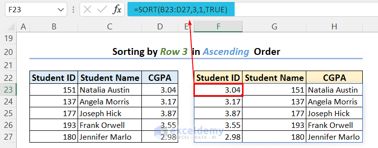
The ascending order of row number 3 is 3.87… 177… Joseph Hick. The whole table is sorted accordingly.
- The SORT function can sort both in alphabetical order and in numerical order. We have sorted the table according to the student names in alphabetically ascending order. The formula for this example is:
=SORT(B32:D36,2,1,FALSE)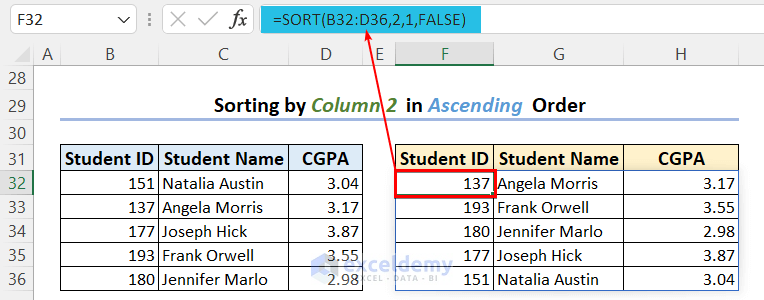
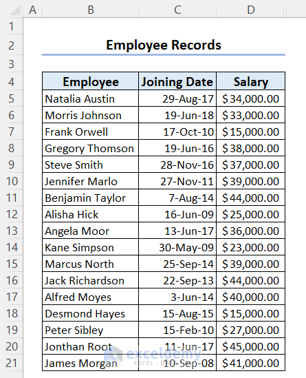
We have the names, joining dates, and salaries of some employees of a company.
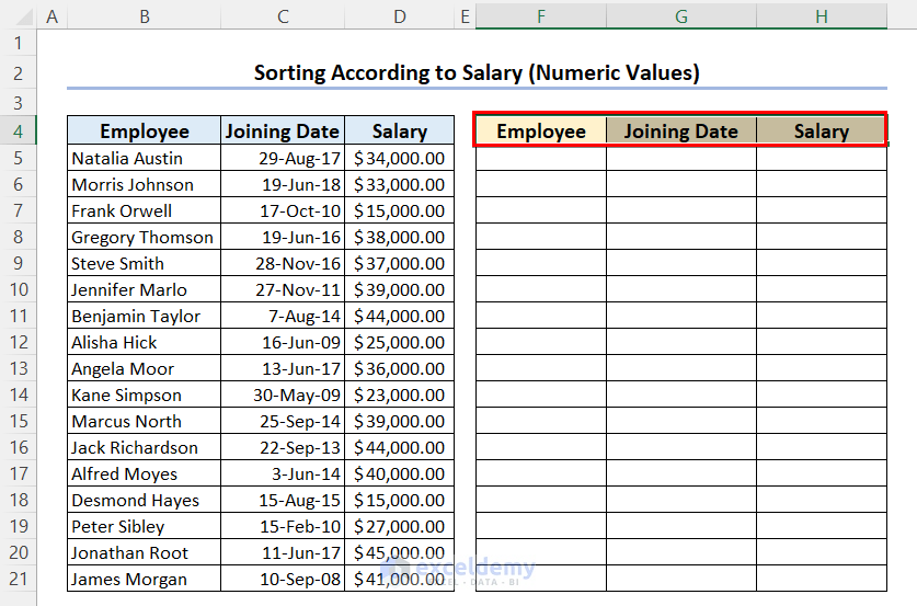
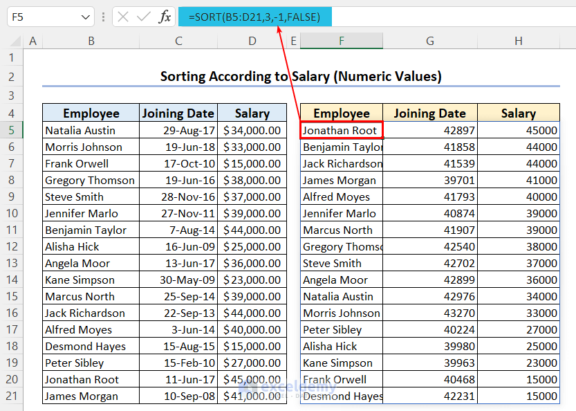
Example 1 – Sorting a Group of Employees According to Their Salaries (Sort by Numeric Values)
We inserted a table to present the results.
- The formula will be:
=SORT(B5:D21,3,-1,FALSE)
Formula Explanation:
- The array argument is the range B5:C21. Sort the cells from this table.
- The sort_index argument is 3. That means the table will be sorted according to the 3rd column or the 3rd row (Depending on the by_col argument).
- The sort_order argument is -1. That means the table will be sorted in descending order.
- The by_col argument is FALSE. That means the table will be sorted through rows, not through columns, according to column number 3.
- The formula SORT(B5:D21,3,-1,FALSE) sorts the array B5:C21 by sorting it through the rows according to column 3 in descending order.
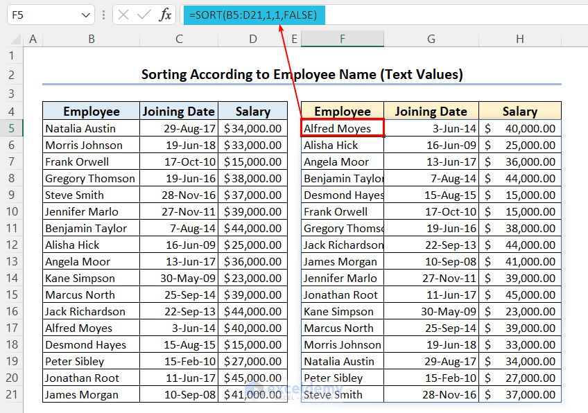
Example 2 – Sorting a Group of Employees According to the Names (Sort Alphabetically)
We will sort the employees according to their names in ascending order.
- Select a new cell and enter this formula:
=SORT(B5:D21,1,1,FALSE)
Formula Explanation:
- The array argument is the range B5:D21. Sort the cells from this table.
- The sort_index argument is 1. That means the table will be sorted according to the 1st column or the 1st row (Depending on the by_col argument).
- The sort_order argument is 1. That means the table will be sorted in ascending order.
- The by_col argument is FALSE. That means the table will be sorted through rows, not through columns, according to column number 1 (Employee Name).
- The formula SORT(B5:D21,1,1,FALSE) sorts the array B5:D21 by sorting it through the rows according to column 1 in ascending order.
Example 3 – Sorting a Group of Employees According to Their Joining Dates (Sort by Date)
- Select the first result cell and enter this formula:
=SORT(B5:D21,2,1,FALSE)
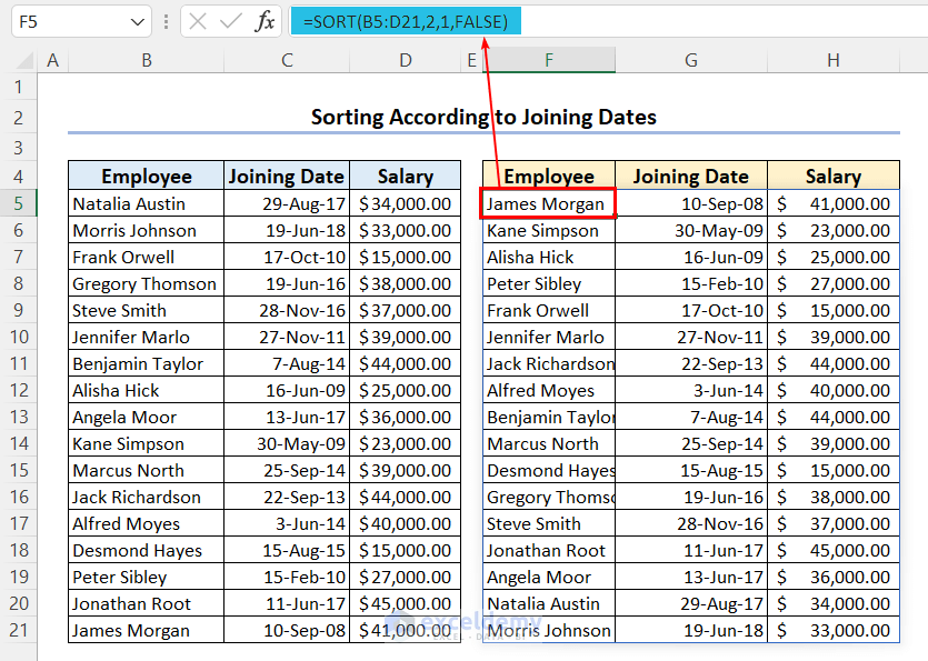
Formula Explanation:
- The array argument is the range B5:D21. Sort the cells from this table.
- The sort_index argument is 2. That means the table will be sorted according to the 2nd column or the 2nd row (Depending on the by_col argument).
- The sort_order argument is 1. That means the table will be sorted in ascending order.
- The by_col argument is FALSE. That means the table will be sorted through rows, not through columns, according to column number 2 (Joining Date).
- The formula SORT(B5:D21,2,1,FALSE) sorts the array B5:D21 by sorting it through the rows according to column 2 in ascending order.
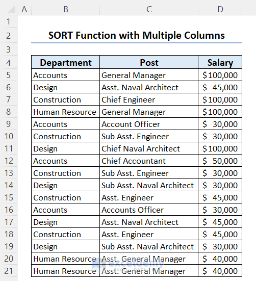
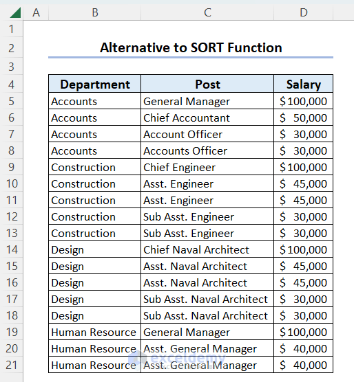
Example 4 – Use the SORT Function to Sort Data in Multiple Columns
We have a salary structure for some positions in different departments in a company. We want to sort it in such a way that we will accumulate the same departments one after another in the column, and then we will sort the salaries of all the positions in each category in descending order (largest to smallest).
- Apply the following formula.
=SORT(B5:D21,{1,3},{-1,-1},FALSE)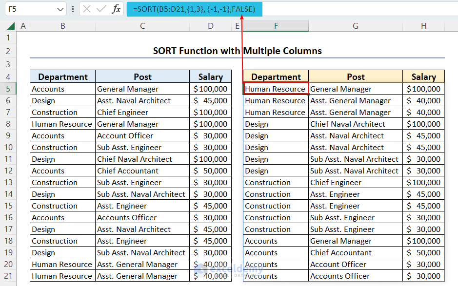
Formula Explanation:
- We have applied {1,3} as sort_index and {-1,-1} as sort_order.
- The SORT function will first count the 1st column as an index to sort data. Also, this sort will be in descending order (descending order has no significance in our case. You could use 1 as sort order too).
- The SORT function will sort the data again considering the 3rd column as sort_index in descending order.
Alternative to the SORT Function for Earlier Versions of Excel
- We have the same data which we have sorted in Example 4.
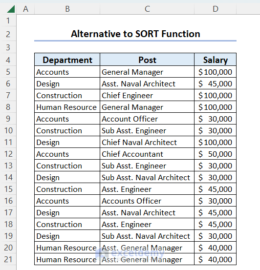
- Select cells B5:D21 and go to the Sort window using the following keyboard shortcut:
- Mark the My data has headers box.
- Go to Options to select sort orientation (top to bottom/left to right). You can relate this with the by_col argument of the SORT function.
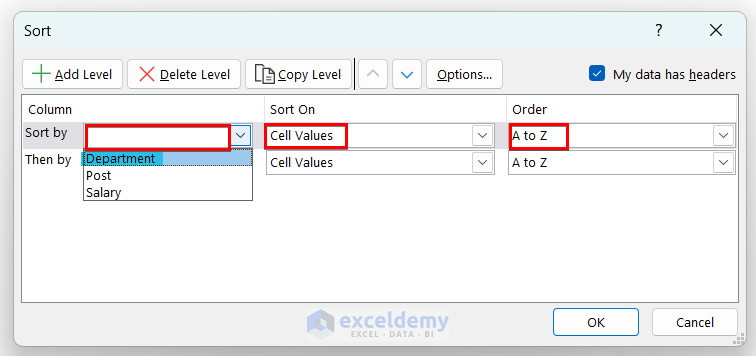
- The Sort option has one sort level by default, but you can add more levels. Since we will sort the data twice (first by department column, then by salary column), we will add one more level.
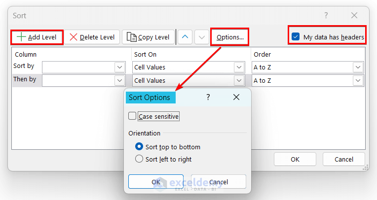
- Click on Sort by and choose a suitable sort index (in our case, department). This parameter is comparable to the sort_index of the SORT function.
- Choose Order A to Z (Ascending order). This is the SORT function’s Sort_order argument. Keep the Sort On option as-is.
- Click on the Then by list and choose the next sort index, i.e. Salary.
- Choose Sort On as Cell Values and pick the Sort Order again. We have picked Largest to Smallest as Order here.
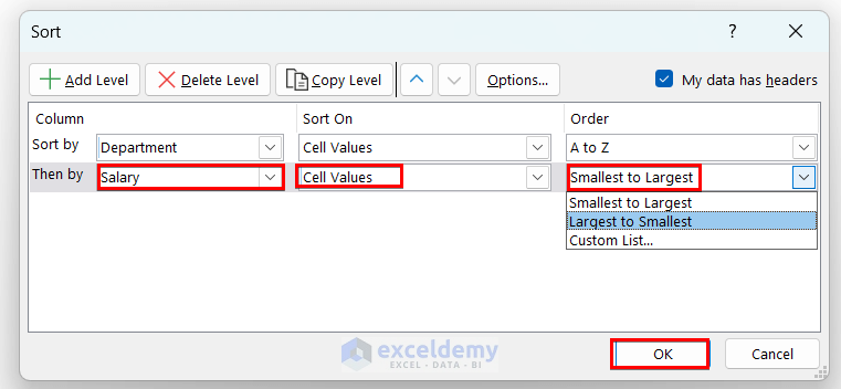
- Press OK.
This is the equivalent of the following SORT formula:
=SORT(B5:D21,{1,3},{1,-1})Limitations of the SORT Function
- You can’t use the SORT function if you want to sort any range of cells according to a row or column outside that range. To solve these types of problems, you can use the SORTBY function of Excel.
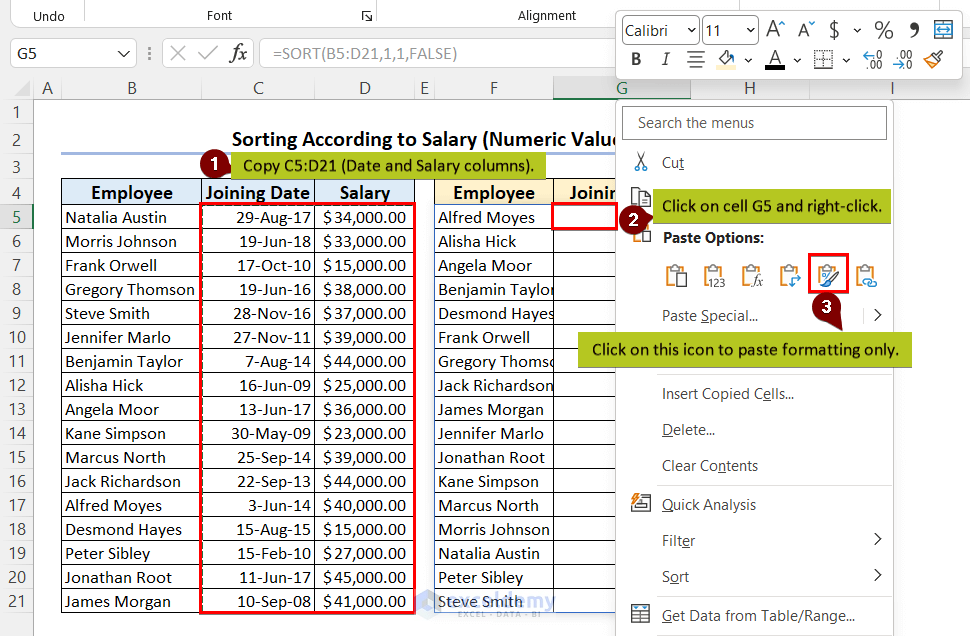
- You may lose the formatting after using the SORT function. To regain the formatting, copy the parent cells that have lost formatting in the new destination, right-click on the upper-left cell of the destination range and, from Paste options, click on the Formatting (R) Icon.
Download the Practice Workbook
<< Go Back to Excel Functions | Learn Excel
Get FREE Advanced Excel Exercises with Solutions!
