Latest Posts From Afrina Nafisa

In this article, we will create a surface chart in Excel. There are four types of surface charts and here we will discuss about 4 of them. Here, we will also ...
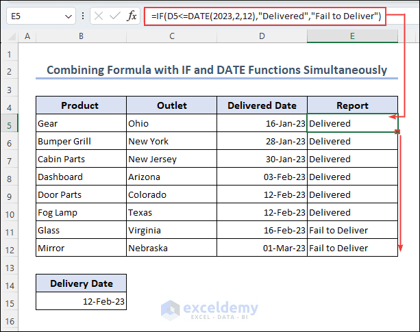
In this Excel tutorial, we will learn how to - Use the combination of the IF and DATE functions along with the combination of the IF and TODAY functions to ...

This is an overview. Download Practice Workbook Hide Cells.xlsx Method 1 - Using the Keyboard Shortcut to Hide Cells Across Columns ...

Here, we will learn how to create hyperlink in Excel using the toolbar, and context menu. Here we also used formulas to create hyperlinks in Excel. Therefore, ...
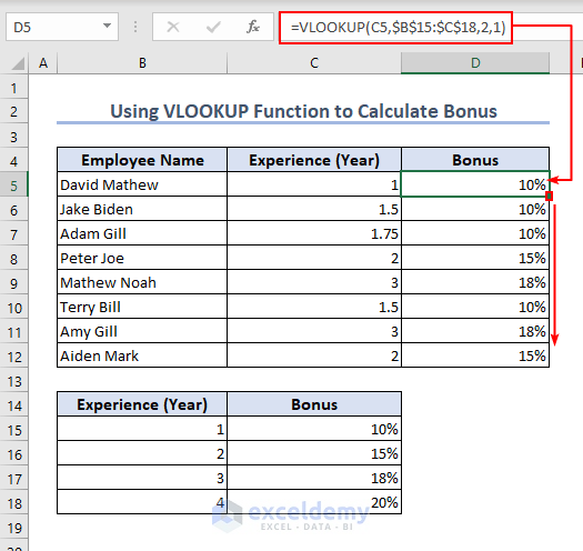
Download Practice Workbook Download the worksheet. Performing VLOOKUP in Range.xlsx Example 1 - Applying the VLOOKUP Function to get ...

In this article, we will learn how to create an Excel array formula. Here we will create an array formula for single-cell and multi-cell values using different ...

Here, we will learn Excel compare columns using different processes and formulas such as conditional formatting, IF function, EXACT function, AND function. We ...

The overview shows the summary of splitting first and last names, separating numbers from text, and splitting cells vertically across rows. Here, the C column ...

Method 1 - Create the Chart in Excel Select the table range C5:D13 and go to Insert Tab >> Chart to create a chart. An Excel Chart is added ...

In this Excel article, we will learn how to calculate non-linear interpolation Excel. While working on a dataset, we need to deal with those data points that ...

In this article, we will get Excel color index numbers using Excel VBA. Here, we will learn how to get color index numbers in Excel and how to change the ...

In this article, we will learn how to use Excel VBA to calculate cell. We will calculate cell, workbook, worksheet, range, and formula using Excel VBA macro. ...

This article will teach us how to create a sole trader bookkeeping Excel. Here, we will create a template and add all the information to complete the template. ...

In this article, we will learn how to compare two Excel sheets and highlight differences using a macro. So, let's start. Sometimes we are working on two ...

This dataset represents sales and profit of different companies over the year. The Office theme was used to create the dataset. Step 1 - Download ...
See Our Reviews at


Hello ROB,
Hope you are doing well. The behavior you describe is how a scanner or browser shows the URL while scanning. The QR codes contain the full URL within them, and the scanner opens the full URL.
However, some scanners display the base domain of the URL for user-friendliness and simplification. Unfortunately, there is no direct solution but you can use online URL decoder to see the encoded URL before opening or try different scanners to get the full URL while scanning the QR code.
I hope this will help you to solve your problem. Please let me know in the comment section if there are any other queries.
Regards
Afrina Nafisa
Exceldemy
Hello RENAE HINES,
Hope you are doing well. Thank you for your query. You can create a dynamic checklist using Excel’s built-in feature such as Data Validation.
=FILTER($C$5:$C$16,EXACT($B$5:$B$16,E5))Hello Rick Howard, Thank you for your query. Therefore, method 3 is updated in the article. Now you may find any champion team or any runner Up team of any random League using The VLOOKUP function and the MATCH function.
Hello JESSPEAR,
Hope you are doing well. In Discount price Column we used formula with relative cell reference that’s why xlPasteFormulas command copying the formula of that column with same cell reference. In Column E you will get the result with relative cell reference.
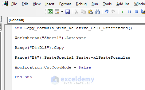
However, you can also use the OFFSET function to copy the formula with relative reference.
Hello FARHAN,
Hope you are doing well. I can see the formula in this article to calculate commission is a bit tricky. However, you can use the below procedure to calculate commission. I believe this formula is easier than the previous one.
=IF(K5< 12%,0,IF(K5 <= 20%, I5 *0.005,I5 *0.015))Here is the final output after applying the formula to calculate the commission.
Hello SHAWN,
Hope you are doing well. Well, you can try the code below to get multiple cells value in pivot table.
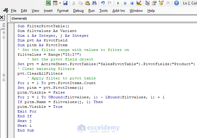
Code
Initially, the pivot table is similar to the below image.
Here is the final output.
Hello Gianluca,
Hope you are doing well. Thank you for your query. Well, I can see two columns here and you need to get the running maximum of the values using a dynamic array. Therefore, you can use the MAX function to get the running maximum from the dataset. You may follow the below image to use the MAX function as an array function. If you use the total column in the formula as below then the formula will work like an array formula. You can add or change any value within the range and the running maximum value will change according to your dataset.
[wpsm_box type="green" float="none" textalign="center"]
=MAX($B:$B,$C:$C)[/wpsm_box]
Here, if add another column then the formula adds the values in the range and changes the output as below.
Hello M,
Thank you for your query. I hope you are doing well. The quickest way to convert CSV files to XLSX files is by using programming languages like Excel VBA. You may check Method 4 ( Applying VBA Code to Convert Multiple CSV Files to XLSX without Opening) to convert multiple files in subfolders.
Hello OLWETU,
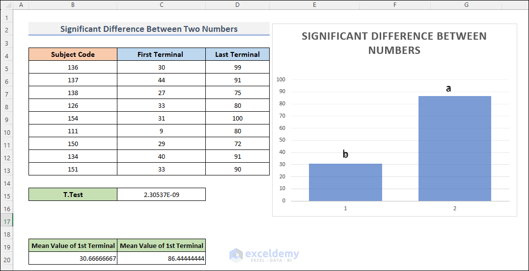
I hope you are doing well. Well, thank you for your query. Adding asterisks to graphs is a significant way to show the difference between two or more groups. You can get the mean value of the treatments using the ANOVA method. Then plot the mean values in the graph. This part is relatively easy and already shown in the article. Now, if you want to add the asterisks to the chart to define the largest mean then select the chart and check the Data levels as below.
Therefore, write down “a” in a cell and double-click the value of the highest mean value. Once you click on the data levels you will see the options of selecting data levels. Finally, select Choose Cell to get the asterisks as “a”.
Now, apply the MIN function to get the minimum value of the mean values and inter asterisks as “b” using the same process.
Hello JACOB FLOYD,
Thanks for your valuable contribution. Now this method is added to this article. Please let us know if you have any queries regarding this article.
Hello, Kevin King. I am glad that you liked this article and this article helped you when you needed the most. Hopefully, we will help you more with our other articles. Please leave a message if there is any other query.
Hello BLAKE HUGUENIN. Thank you for your query. I believe the best way to combine multiple spreadsheets and pivot tables is using Power Query. Please follow the below steps:
Initially, select Data >> Get Data >> From File >> From Excel Workbook Toolbar.
Now, Get the Import File dialog box and select the required file.
Then navigator tab will be visible and select the worksheet to copy the sheet in another workbook. Complete the process by clicking on Load and Close.
Now repeat this process to add sheets as much as you want. Using Power Query is better because if you change the value in any of the workbooks then the value will be changed in master workbook.
Now, if you want to create a dashboard that will be dynamic and change the values of the data if the primary data is changed then use formula =(Sheetname!Range) in the dashboard. For instance =(File4!C5:C13). Please find Add Multiple Worksheets in the master workbook
Hello, NARASIMHAN S
Please find the below code to get only specific sheets by name.
Note: Change the Path Id and the sheet name according to your convenience.
Hello, CALEB HOGUE. Thank you for your query. I understand you find difficulties using 9 and 10 as Tab and Enter. Please follow the below code to get 9 and 10 as Tab and Enter respectively.
Sub ActivateFirstBlankCell()
Dim cell As Range
Also, follow the code that is already used in this article to convert “8233 CR 8233 CR” into one barcode
Hello ERIC. Thank you so much for your query. Please follow the formula below to get the days between the two dates, including the Launching and Closing dates.
=IF(NETWORKDAYS.INTL(C5, D5, 1) > 0, NETWORKDAYS.INTL(C5, D5, 1) + 1, IF(WEEKDAY(C5, 1) < WEEKDAY(D5, 1), NETWORKDAYS.INTL(C5, D5, 1) + 2, NETWORKDAYS.INTL(C5, D5, 1) + 1))Here, we used NETWORKDAYS.INTL function along with the IF function. Now, this formula can check if the launching date or the closing date is a weekend and adjust the result accordingly. For a better understanding, you can check Number-of-Days-Between-Two-Dates-Calculator-1 as well.
Hello, JACK LONETTO. Thank you for your query. After calculating the loan installment using Amortization Schedule with your given criteria, it shows the loan will be dismissed after the 6th installment if you go with a 20% down payment at the beginning of the year.
If you want to complete this process in 10 years then the criteria will be-
Amount Financed $5,280,000
Interest Rate 4%
Term 10Years
At the beginning of Year2 2% Down payment
At the beginning of Year3 2% Down payment on the Remaining Balance
At the beginning of Year4 2% Down payment on the Remaining Balance
At the beginning of Year5 2% Down payment on the Remaining Balance
At the beginning of Year6 2% Down payment on the Remaining Balance
At the beginning of Year7 2% Down payment on the Remaining Balance
At the beginning of Year8 3% Down payment on the Remaining Balance
At the beginning of Year9 3% Down payment on the Remaining Balance
Remaining balance at the beginning of year10
For a better understanding, you can check Amortization-Schedule-with-Irregular-Payments as well.