Method 1 – Insert a Pivot Table
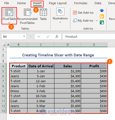
- Select the data range B4:E13 to build the pivot table
- Select Insert >> PivotTable from the Toolbox as below.
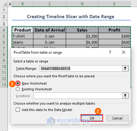
- Pivot Table from Table or Range dialog box will appear as below.
- Select New Worksheet so that, the pivot table appears in another sheet, and select OK to complete this process.
Method 2 – Add Fields to the Pivot Table
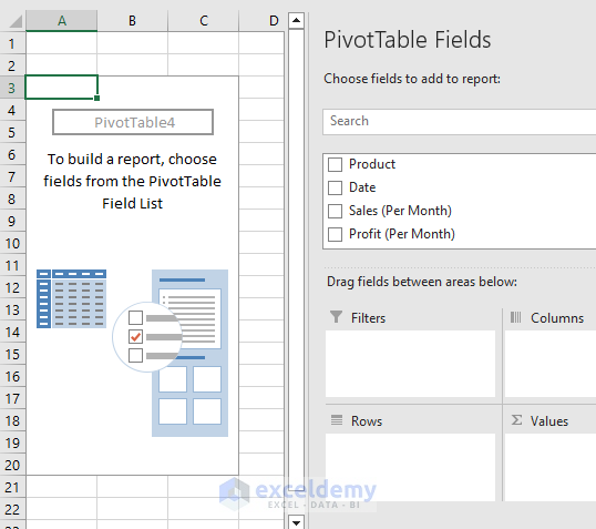
- Once the OK option is clicked, the structure of the pivot table will appear in another sheet.
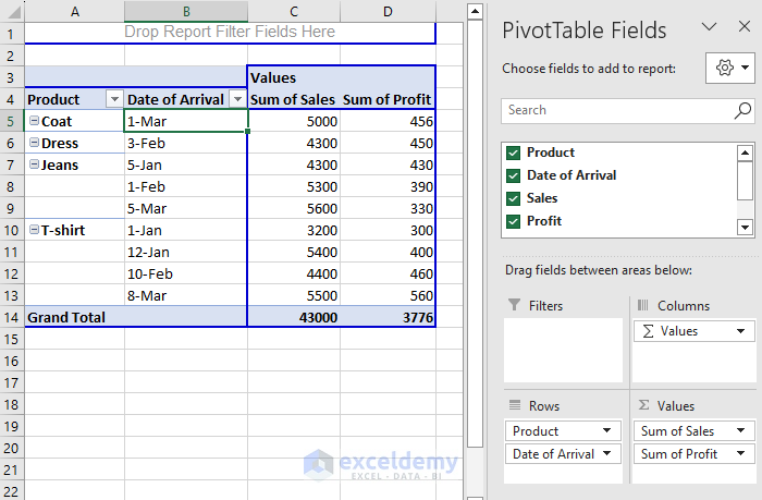
- Select the required fields from the PivotTable Fields and the pivot table is complete.
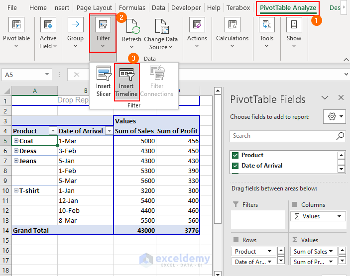
Method 3 – Add Timeline Slicer for Date Range
- Select Pivot Table Analyze >> Filter >> Insert Timeline from the ribbon.
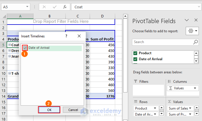
- The Timeline dialog box will appear.
- Select Date of arrival from the dialog box and click OK.
Method 4 – Final Output
- The Timeline slicer will appear like the picture below.
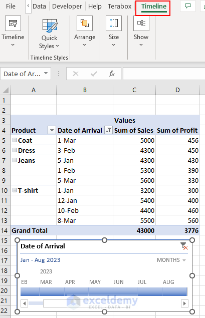
- Now, select the area to get the required result.
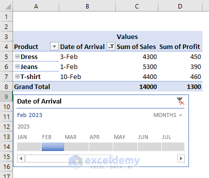
Note: You can change the selected area according to your requirement and filter the data of the dataset as required.
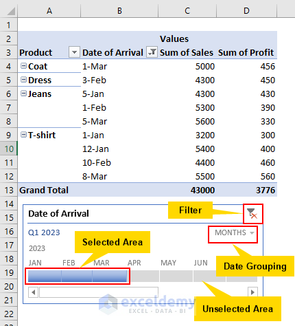
- Selected Area: This is the required area of data. Once you select a particular area, the data of that area is shown as output.
- Unselected Area: This is the muted area. If you don’t need data from a particular area, unselect it.
- Filter: Filters the data from the Date of Arrival option.
- Date Grouping: Represents the time period of the data. If the data represents Year, it shows year in date grouping. If the data represents Month, represents month.
How to Remove Timeline Slicer in Excel
- Select the Timeline slicer and right-click the mouse to open the menu.
- Select Remove Timeline from the menu bar and remove the timeline slicer if it is unnecessary.
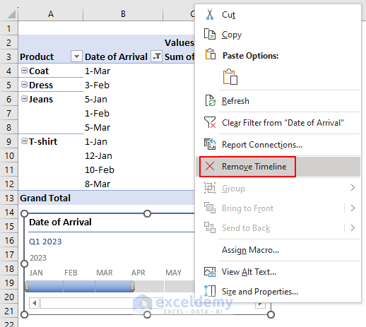
Note: Or select the timeline slicer and press the Delete key on the keyboard.
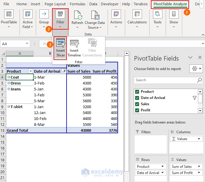
How to Add a Slicer to a Pivot Table in Excel
- Select Pivot Table Analyze >> Filter >> Insert Slicer from the toolbox.
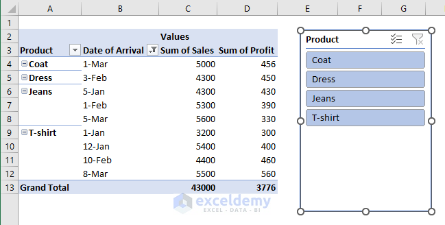
- Insert Slicer dialog box will pop up as before, and select the required field (For instance, select Product).
- Once you select Product click OK.
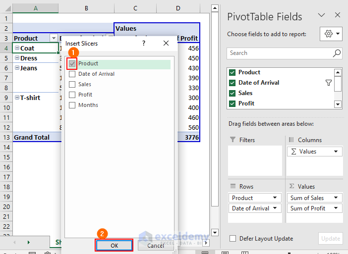
Note: You can choose one single option or multiple options at a time.
- The slicer will pop up and choose according to the requirement.
Things to Remember
- A timeline slicer is used when we need to filter the data according to the date. Otherwise, the timeline slicer will not work.
- You can select multiple fields at a time while using a timeline slicer.
Download Practice Workbook
You can find the practice workbook here.
Further Readings
- How to Create Slicer Drop Down in Excel
- How to Custom Sort Slicer in Excel
- Excel Slicer Vs Filter (Comparison & Differences)
- How to Make Excel Slicer with Search Box

