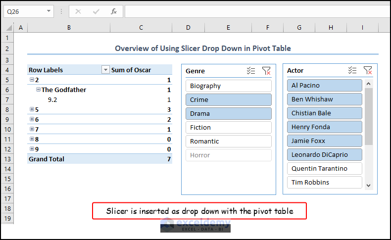
With the slicer drop-down, you can quickly and easily filter data by selecting one or more items in the drop-down list, which instantly updates the pivot table or chart. Consider the following dataset where a slicer can effectively filter movies by genre and actors.
What Is a Slicer Drop Down in Excel?
Slicers provide a visual way to filter data by displaying buttons or drop-down lists that correspond to specific data sets. When a user selects an item in the slicer, it filters the pivot table or chart based on that selection, allowing for quick and easy data analysis.
How to Create a Slicer Drop Down in Excel: with Quick Steps
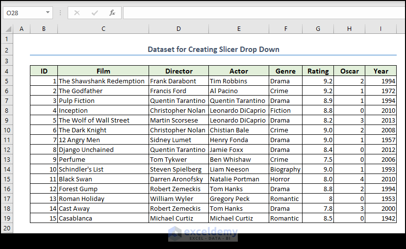
- Create a dataset to prepare the pivot table. We have included a dataset containing Film, Director, Actor, Genre, Rating, Oscar, and Year columns.
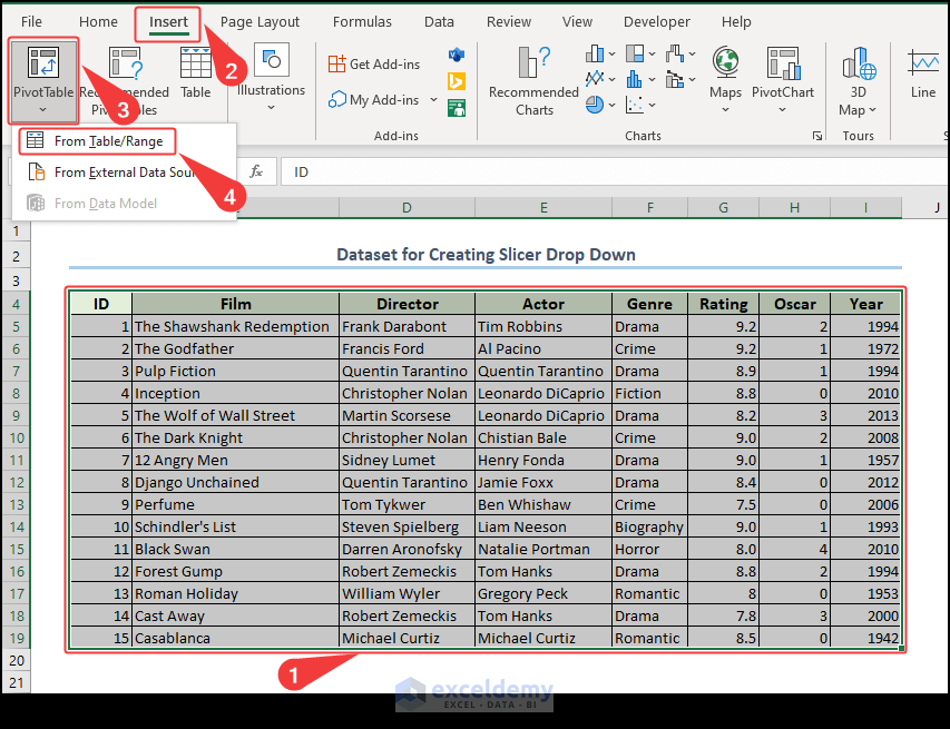
- Select the whole data table including the headers.
- Select Insert, go to Pivot Table, and choose From Table/Range.
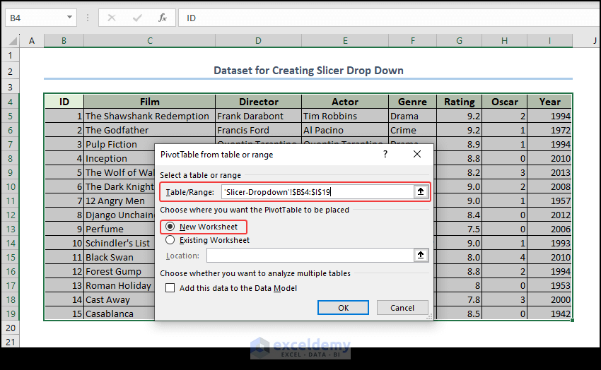
- A Pivot Table from table or range tab will appear. Check the input range (which should be filled up automatically).
- Click on New Worksheet to create the table in a new worksheet.
- Click on the pivot table object, and pivot table fields will appear on the right pane.
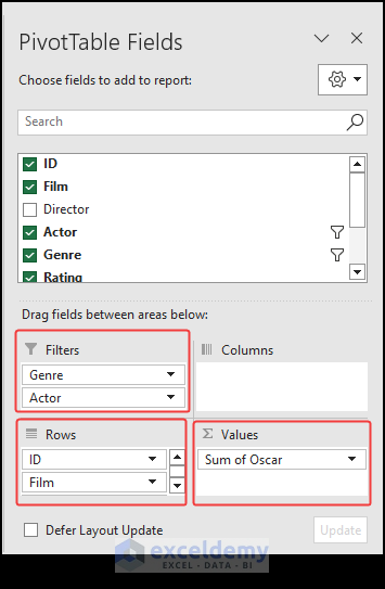
- Put the fields ID and Film in the Row section, and put the Oscar field in the Values section.
- Take the fields Genre and Actor in the filter section.
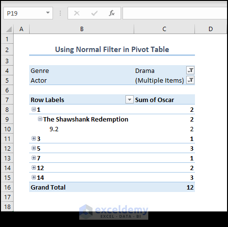
- We will see the pivot table with filters like in the image given below.
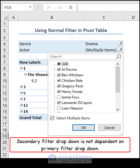
- Select different items from Genre filter. Check the Actor filter which is unaffected by the change in Genre filter selection.
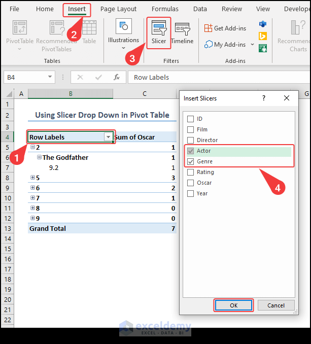
- Click on the pivot table.
- Select Insert and then Slicer (from the Filters section).
- Select the item from the checklist to add as Slicer. We have selected Genre and Actor.
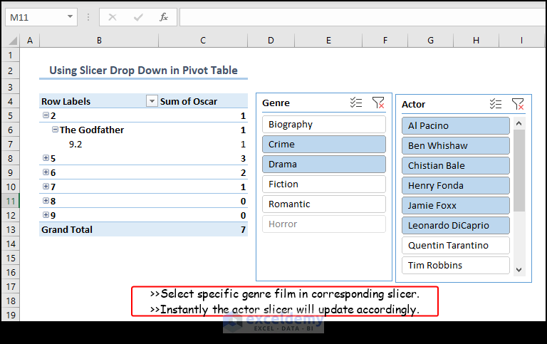
- You will get the slicer included in the pivot table sheet. Select some items from the Genre slicer and see if the items from the Actor slicer adapted accordingly.
How to Customize a Slicer Drop Down in Excel
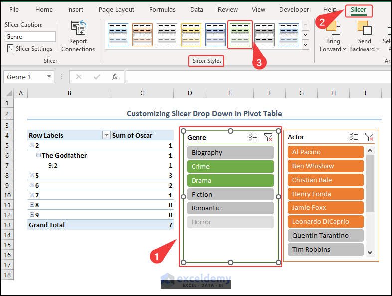
Method 1 – Changing Slicer Style
- Select the slicer.
- Select the Slicer tab in the top ribbon and pick your desired style for the slicer from the list.
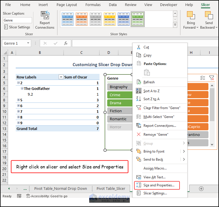
Method 2 – Change the Size and the Properties of a Slicer
- Right-click on the slicer and select Size and Properties.
- Change the size and properties of the slicer from the right pane according to your needs.
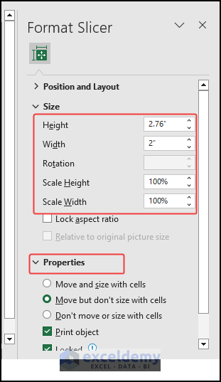
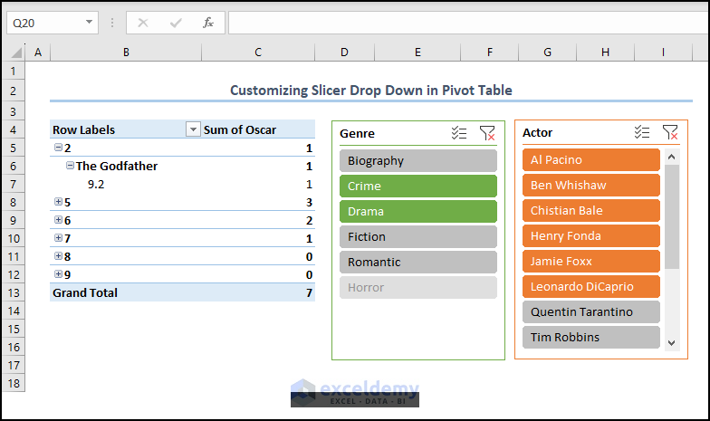
- You will get a customized slicer like in the image below.
Read More: How to Custom Sort Slicer in Excel
What Are the Advantages of an Excel Pivot Table Slicer Over a Normal Drop Down?
- Visual Filtering: Slicers provide a visual representation of the data filters that are being applied to the pivot table. This makes it easier to see the filters that are currently in effect and to make changes as required.
- Multiple Selections: Unlike drop-down lists (generally), slicers allow users to select multiple items at the same time. This can be very useful when analyzing large datasets with multiple categories.
- Easy to Use: Slicers are very user-friendly and intuitive. Users can simply click on the items they want to filter and the pivot table will update automatically.
- Customizable: Slicers can be customized to match the look and feel of the data analysis report, making it easier to create professional-looking reports.
- Easy to Create and Manage: Slicers can be created and managed with just a few clicks in Excel, making them a quick and easy way to filter data.
Frequently Asked Questions
What is the difference between a slicer and a filter in Excel?
A slicer is a visual filtering tool in Excel that is used to filter data in a pivot table or pivot chart. A filter is a more general term that can refer to any tool or technique that is used to narrow down data in Excel.
Can I use a slicer with non-pivot table data?
No, slicers are designed specifically for use with pivot tables and pivot charts in Excel.
How do I remove a slicer in Excel?
Go to the “Slicer Tools” tab and click on “Remove Slicer.”
Things to Remember
- Change the field elements in the Row, Column, Values, and Filters section from the pivot table pane in the pivot table sheet according to your needs.
- We have included two slicers, you can create more if needed.
- Don’t forget to include the header of the data table before creating the pivot table.
Download the Practice Workbook
Related Articles
- How to Make Excel Slicer with Search Box
- Excel Slicer Vs Filter (Comparison & Differences)
- How to Create Timeline Slicer with Date Range in Excel

