The Slicer provides buttons to filter Excel tables or pivot tables. The visual properties of the slicer such as the size, style, and position of the buttons can be modified, but the contextual tool for resizing a slicer in Excel is limited. However in this article, we will demonstrate an effective way to resize a slicer in Excel.
How to Insert a Slicer in Excel
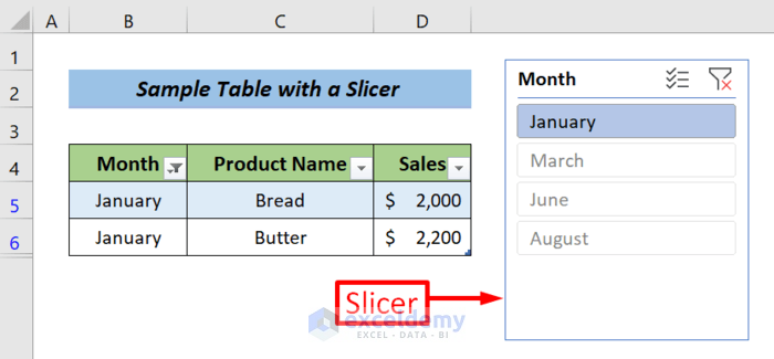
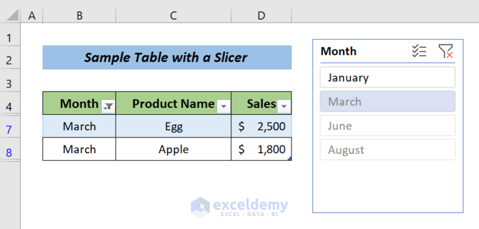
The slicer contains a particular field. For example, the following figure shows a table with a slicer with the heading Month. If we click on January, it will filter only the sales data for January.
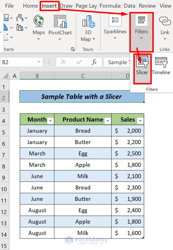
To add one or more slicers in your Excel spreadsheet:
- Select any cell of your table or pivot table.
- Go to Insert >> Filter >> Slicer.
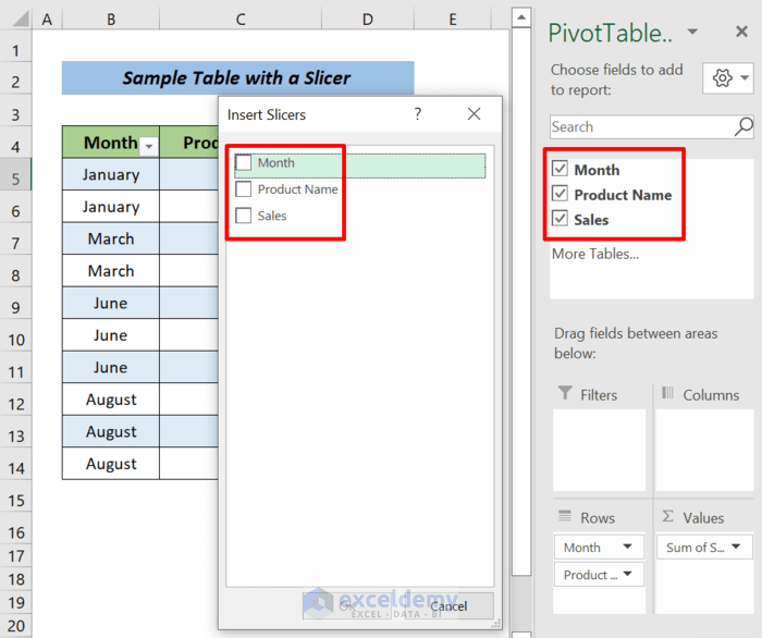
The Insert Slicers dialog box will pop up, including a list of all fields in your table / pivot table.
- Put a checkmark next to one or more fields.
- Click OK.
Read More: How to Insert Slicer in Excel
How to Resize a Slicer in Excel
To resize a Slicer, we’ll create a custom Slicer style.
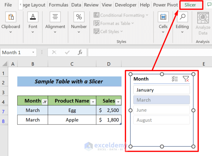
Step 1 – Reveal the Slicer Tab
Select the slicer to reveal the Slicer tool in the ribbon.
Step 2 – Choose a Suitable Style
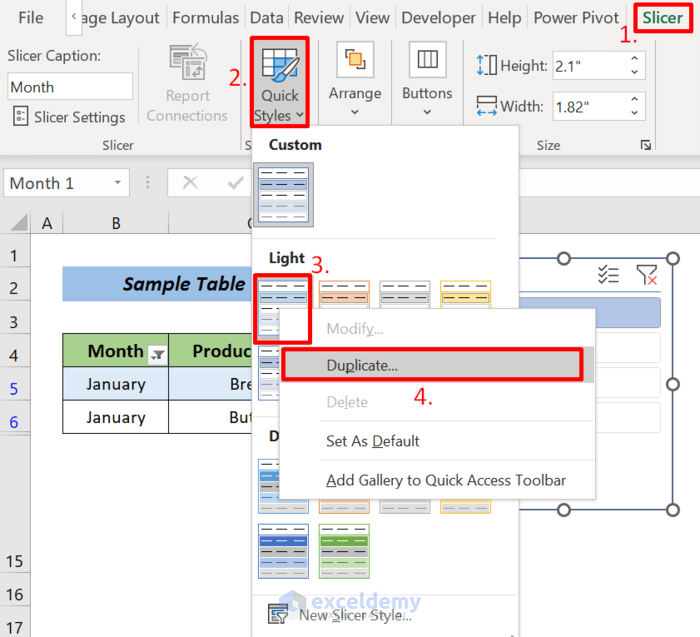
- Go to Slicer >> Quick Styles.
- Choose a style.
- Right-click on the selected style.
- Click on Duplicate.
Read More: How to Change Slicer Color in Excel
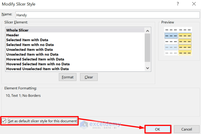
Step 3 – Name the Style
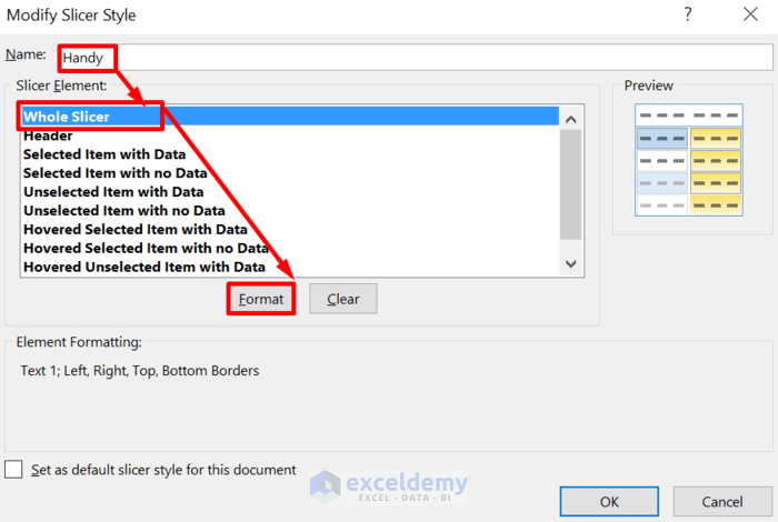
The Modify Slicer Style dialog box opens.
- Give a name to the style (in this example, ‘Handy’).
- Select Whole Slicer from the Slicer Element list.
- Click on Format.
Step 4 -Modify the Font Section to Resize the Slicer
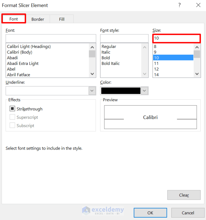
A Format Slicer Element window will pop up.
In the Font tab, select your desired font size and any other elements you wish to modify. Here, we select font size 10 which will reduce the size of the slicer button.
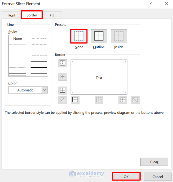
Step 5 – Modify the Borders
- Go to the Border tab and set the Presets to ‘None’, which allows the slicers to overlap slightly.
- Click on OK.
Read More: How to Format Slicer in Excel
Step 6 – Final Tweaks
The Modify Slicer Style dialog box is back.
- Select other slicer elements and modify them as desired.
- Tick Set as default slicer style for this document.
- Click on OK.
The slicer buttons are resized and reformatted.
Download Practice Workbook
Related Articles
- Excel Slicer for Multiple Pivot Tables (Connection and Usage)
- Connect Slicer to Multiple Pivot Tables from Different Data Source
- How to Insert Slicer without Pivot Table in Excel
- [Fixed] Report Connections Slicer Not Showing All Pivot Tables

