To filter and analyze data Excel Slicer helps a lot because it provides some extra features than the Filter command. But the problem is you can’t use Slicer without Pivot Table. So, if you want to ignore Pivot Table then you will have to use it with Table. In this article, I’ll show the easiest way to insert a slicer in Excel without a Pivot Table.
What Is Slicer in Excel?
Slicer is a kind of filter command in Excel that only works in Table and Pivot Table. It not only filters but also allows you to display the filtered data in different sliced sections. It’s quite helpful for a large dataset.
Simple Way to Insert Slicer without Pivot Table in Excel
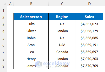
We’ll use the following dataset to show the method that represents some salesperson’s Sales in different Regions.
Insert Slicer Using Table
As I told you before, we can’t insert Slicer without a Pivot Table. So, if you want to ignore the Pivot Table then you must have to use Table. Now, let’s see how to do it using Table.
Steps:
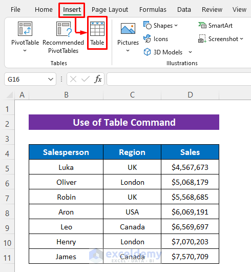
- Select any data from your table and click as follows: Insert > Table.
Or you can press the shortcut key- CTRL + T to insert a table.
- It will automatically select the data range of your dataset. Mark My table has headers if your dataset has headers.
- Then, just press OK.

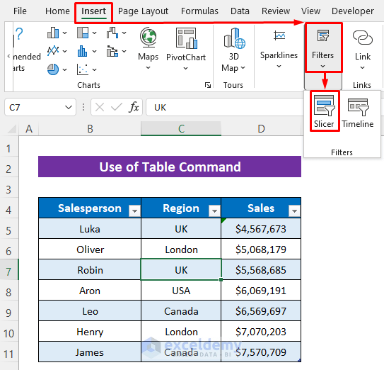
Our table is ready, now we’ll insert Slicer.
- Select any data from the table and then click as follows: Insert > Filters > Slicer.
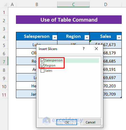
Soon after a dialog box named ‘Insert Slicers’ will appear.
- It will show the headers of your dataset, and mark the headers that you want to get in Slices. I marked Salesperson and Region.
- Next, press OK.
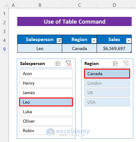
Now, have a look, The Filter icon has appeared in the headers of the dataset and the Salesperson and Region columns have appeared in Slicer.

Now, if you click any value in any Sliced column then the dataset will be filtered according to that value. I clicked Leo so the dataset is only showing Leo’s data in the dataset and Slicer.
- Now, if you want to close the filter from the slicer then just click the Clear Filter icon.
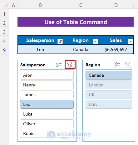
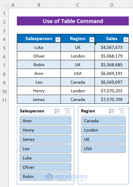
We got back the unfiltered data.
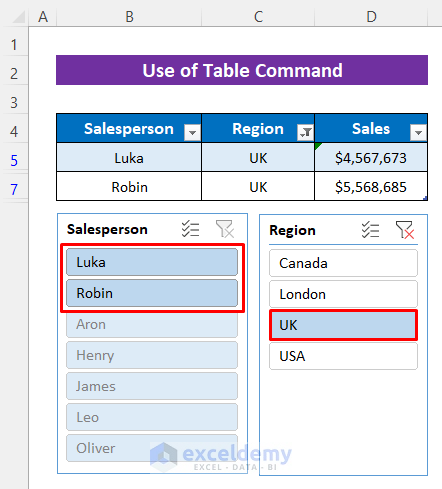
- Now, if you click on the UK from the Region slicer, it will show the corresponding salespersons’ names in the Salesperson slicer along with the filtered dataset.
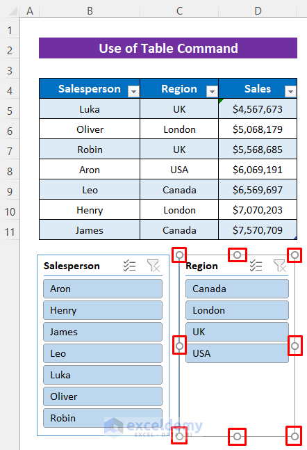
- We can change the position of a Slicer by dragging it with a mouse and can change the size by dragging the circle icon located along the border of the Slicers after clicking on it.
Look, I increased the size of the Region slicer along the right side.

Check the following image to understand how you can do that as well.
Download Practice Workbook
You can download the free Excel workbook from here and practice on your own.
Conclusion
I hope the procedures described above will be good enough to insert the slicer in Excel without a pivot table. Feel free to ask any question in the comment section and please give me feedback.
Related Articles
- How to Change Slicer Color in Excel
- How to Resize a Slicer in Excel
- How to Format Slicer in Excel
- Connect Slicer to Multiple Pivot Tables from Different Data Source
- [Fixed] Report Connections Slicer Not Showing All Pivot Tables
- Excel Slicer for Multiple Pivot Tables (Connection and Usage)

