Dataset Overview
Slicers are powerful tools that allow you to filter data visually, making it easier to analyze and explore your datasets.
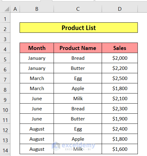
We’ll use the following Product List table, containing the Month, Product Name, and Sales columns, to demonstrate how to insert a Slicer.
Method 1 – Using a PivotTable Fields List
Step 1 – Inserting a Pivot Table
- Open your Excel workbook containing the dataset you want to work with.
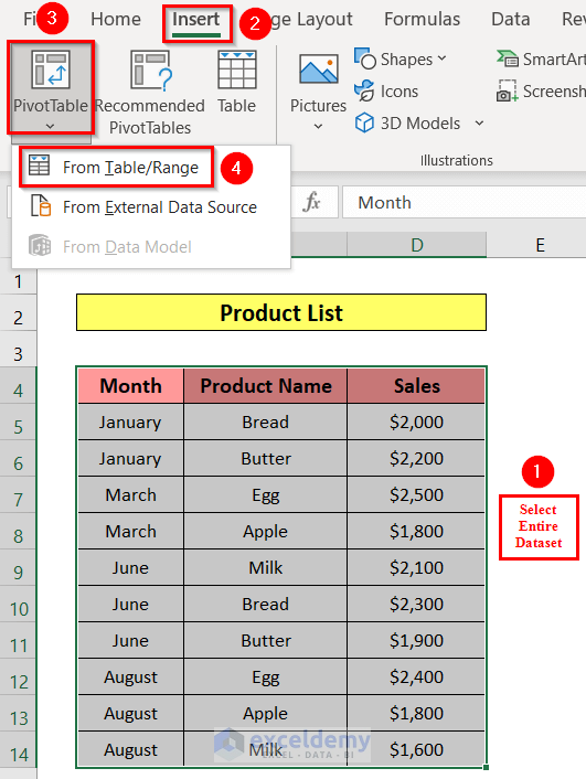
- Select the entire dataset of the Product List table.
- Go to the Insert tab, choose PivotTable and click on From Table/Range.
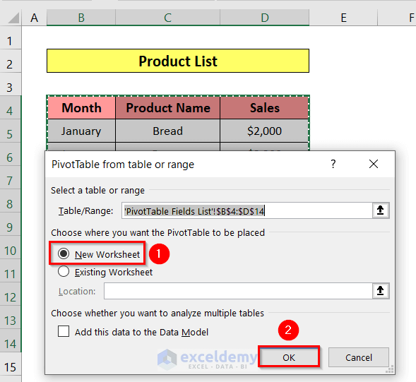
- In the resulting window, click New Worksheet and then OK.
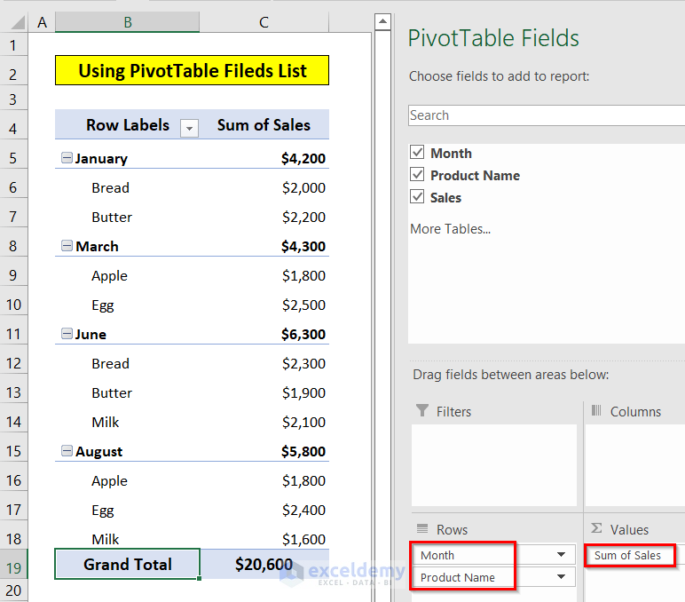
- In the PivotTable Fields, place Month and Product Name in the Rows area, and Sales in the Values area.
- You’ll now have a Pivot Table displaying Row Labels and the Sum of Sales.
Step 2 – Inserting a Slicer Using PivotTable Fields List
- Right-click on any of the PivotTable Fields items (e.g., Product Name).
- Select Add as Slicer.
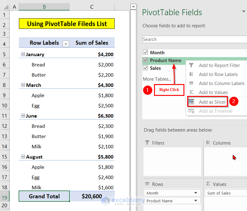
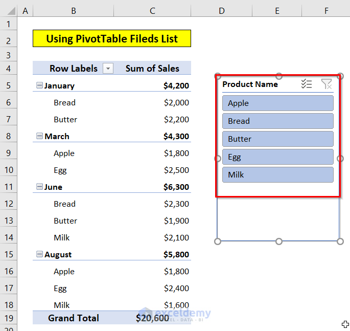
- A slicer will appear, showing a list of Product Names.
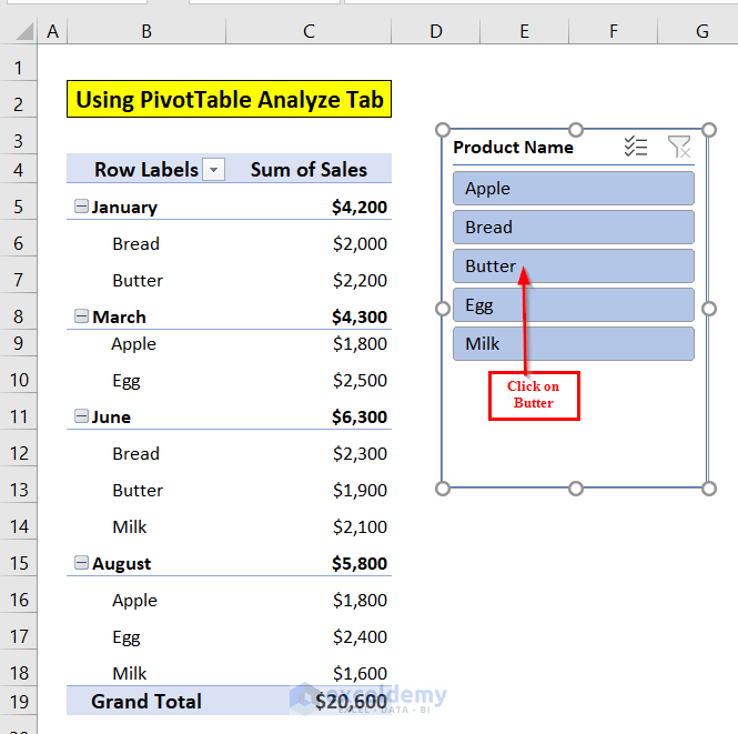
- Click on any Product Name to activate the slicer filter (e.g., select Butter to filter data for that product).
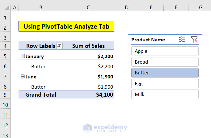
The data for the product Butter is displayed in the Pivot Table.
Read More: Excel Slicer for Multiple Pivot Tables (Connection and Usage)
Method 2 – Using PivotTable Analyze Tab
Step 1 – Inserting a Pivot Table
- Inserting a Pivot Table (same as in Method 1).
Step 2 – Inserting a Slicer Using PivotTable Analyze Tab
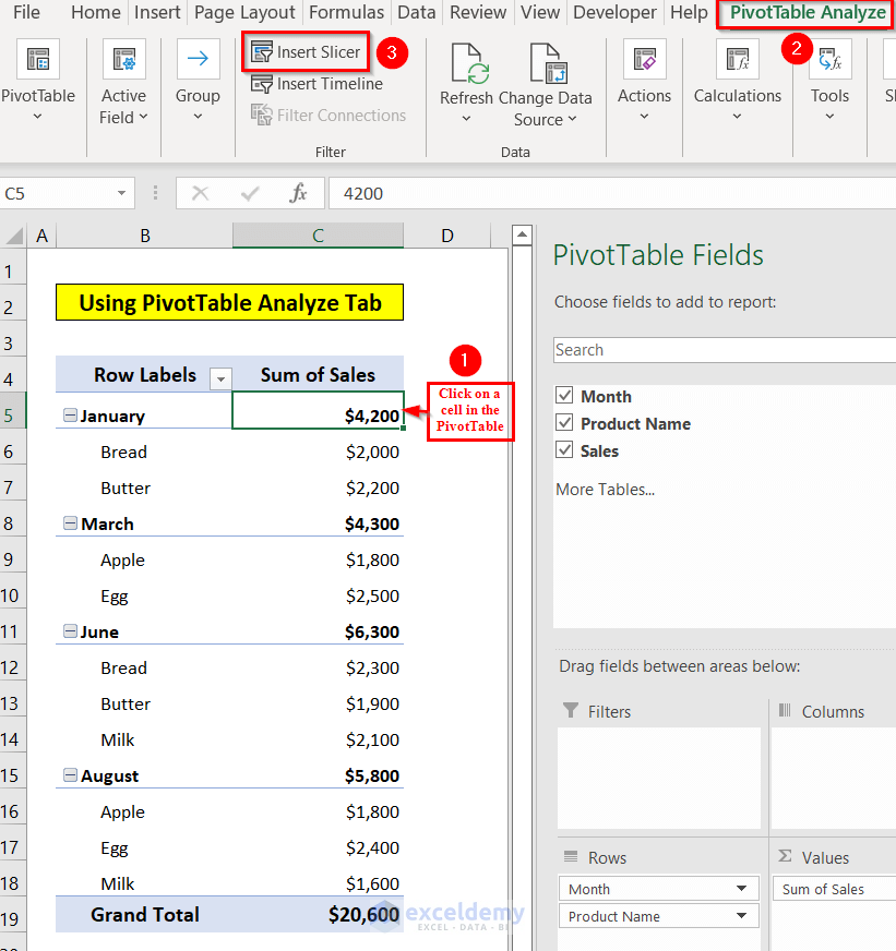
- Click on a cell within the Pivot Table.
- Go to the PivotTable Analyze tab.
- Select Insert Slicer.
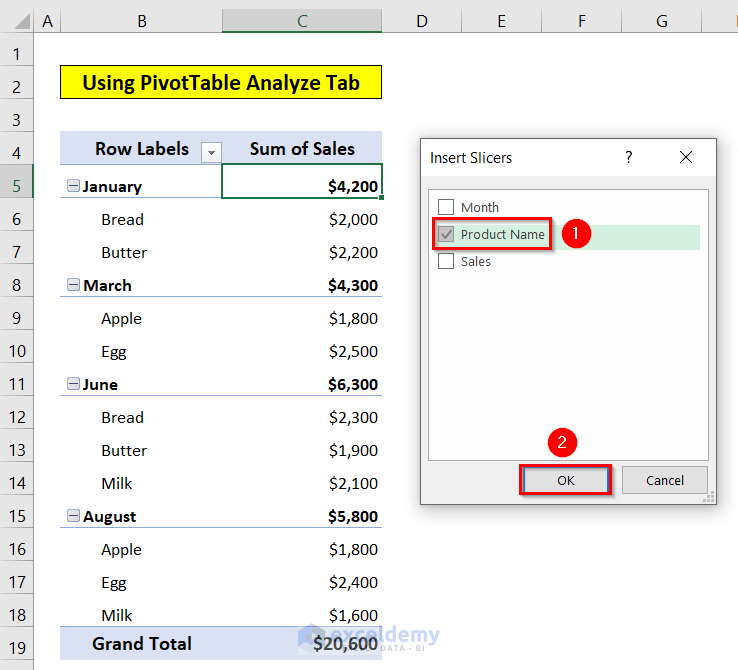
- In the resulting window, choose the field (e.g., Product Name) for which you want to add a slicer.
- Click OK.
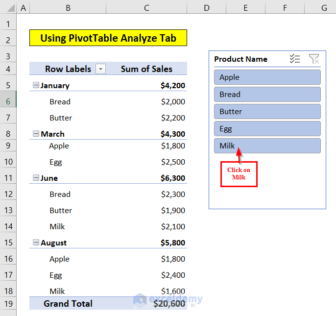
- Now you can use the slicer to filter data based on the selected product (e.g., choose Milk to view data for that product).
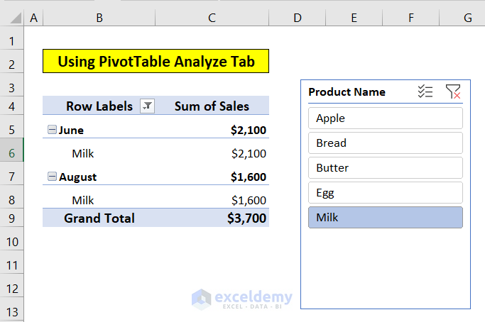
Herewith the data for the product Milk in the Pivot table.
Read More: How to Format Slicer in Excel
Method 3 – Adding a Timeline (for Date Fields)
Step 1 – Inserting a Table
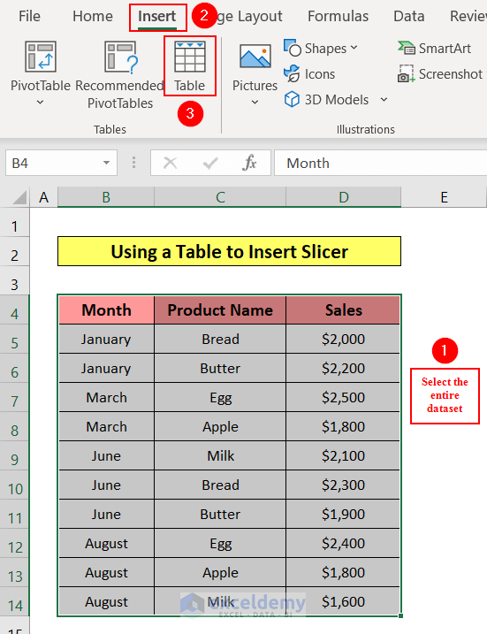
- Select the entire dataset.
- Go to the Insert tab and choose Table.
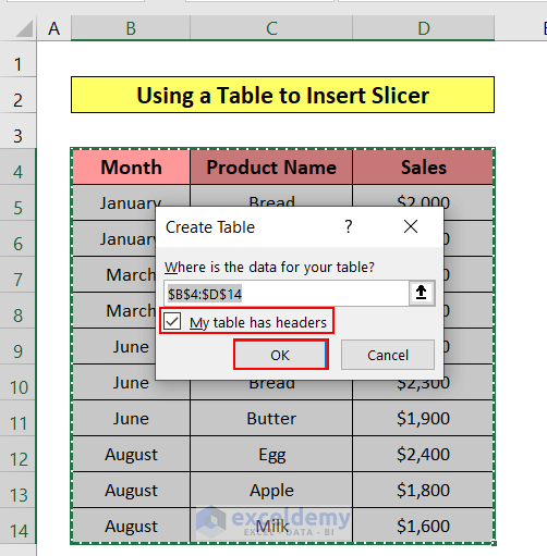
- A Create Table window will appear.
- Mark the My table has headers box and click OK.
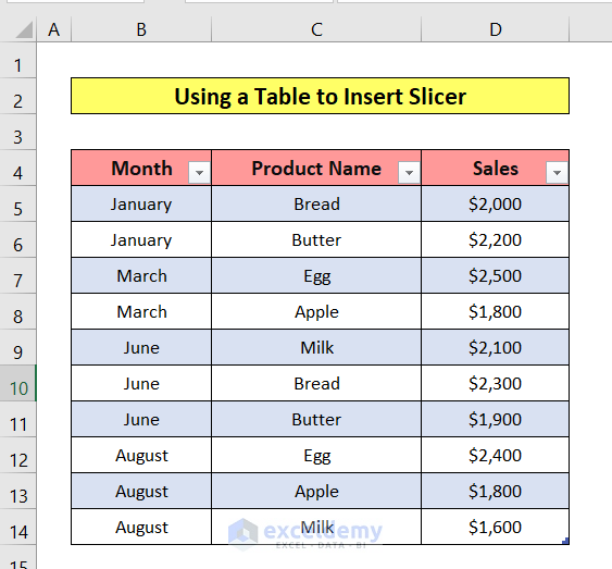
- Now you’ll see the table.
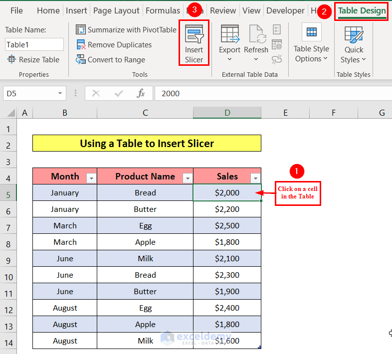
Step 2 – Inserting a Slicer by Using Table Design Tab
- Click on any cell in the table.
- Navigate to the Table Design tab.
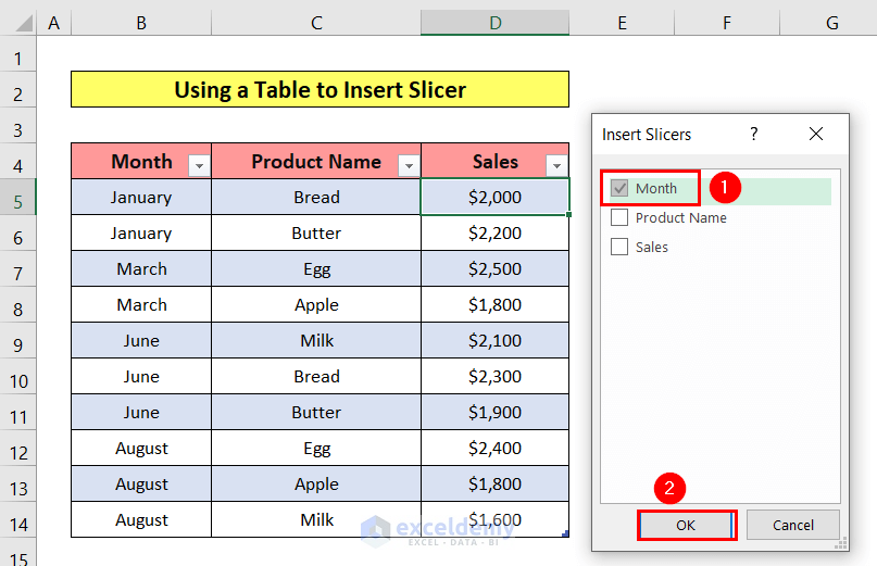
- Select the Insert Slicer option.
- An Insert Slicer window will appear.
- From that window, choose the Month option (you can select other items as well).
- Click OK.
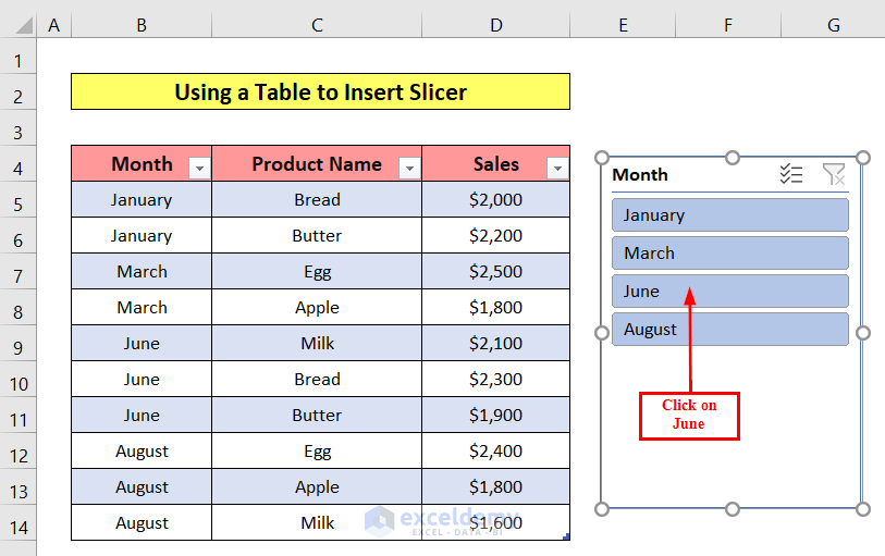
- The Month list will be visible.
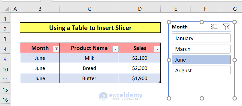
- To filter data for a specific month (e.g., June), click on that month.
- You’ll now see the data for June in the table.
Download Workbook
You can download the practice workbook from here:
Related Articles
- How to Change Slicer Color in Excel
- How to Resize a Slicer in Excel
- Connect Slicer to Multiple Pivot Tables from Different Data Source
- How to Insert Slicer without Pivot Table in Excel
- [Fixed] Report Connections Slicer Not Showing All Pivot Tables

