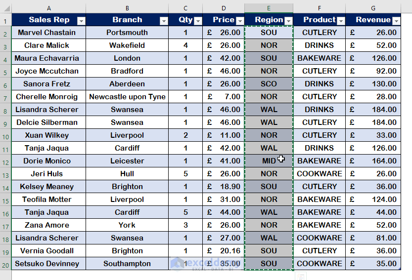
We’ll link a slicer between two data sets in the sections below. The first data set is for the sales data in the Sales worksheet, and the second data set is for the returned products from the sold products in the Returns worksheet. Using the data from the Sales and Returns worksheets, we’ll build a new worksheet for the corresponding value in Region. We’ll put them in a separate worksheet labeled Region. Then, we’ll combine the Sales and Returns data into two pivot tables in the same spreadsheet. We’ll connect the slicer for Region values to the two pivot tables and analyze the data for Sales and Returns Values.
Step 1 – Create a Table with Sales Data
- In the Sales worksheet, select a cell.
- Press Ctrl + T to create a table.
- Select the data range with the column header.
- Click OK.
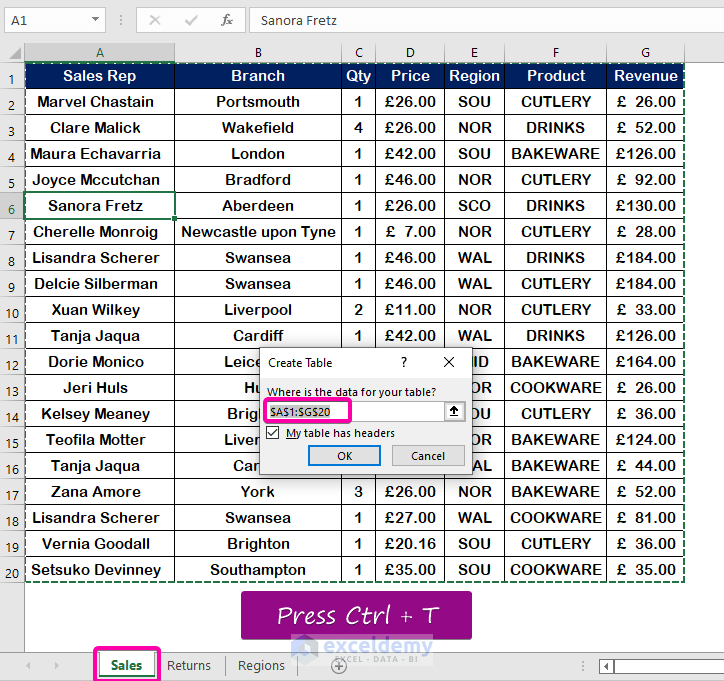
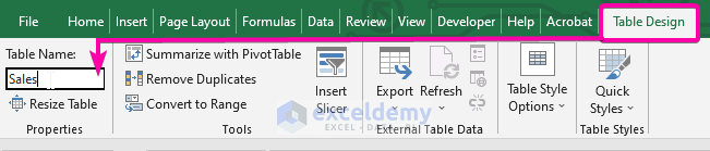
- Name the table as Sales.
Step 2 – Create a Table with Return Data
- In the Returns worksheet, select a cell.
- Press Ctrl + T to create a table.
- Click OK after selecting the data range with the column header.
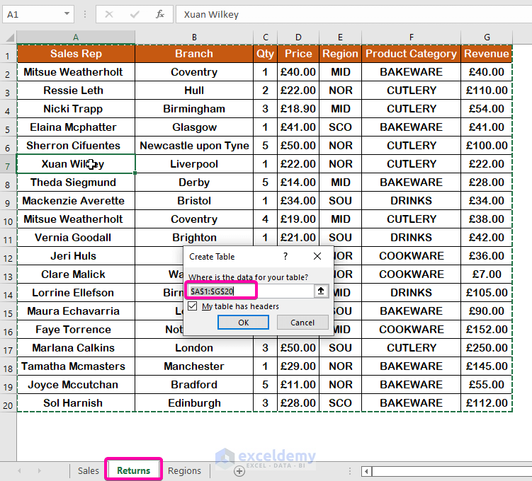
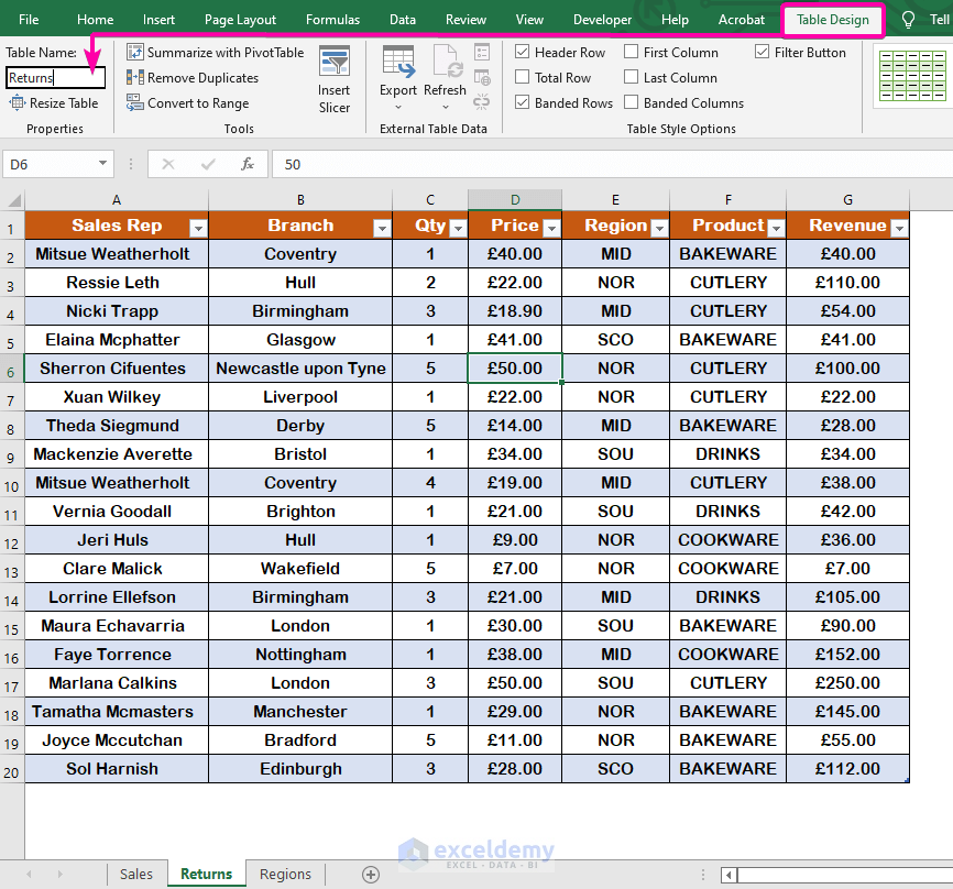
- Give a name (Returns) to the table.
Step 3 – Create a Table for the Slicer
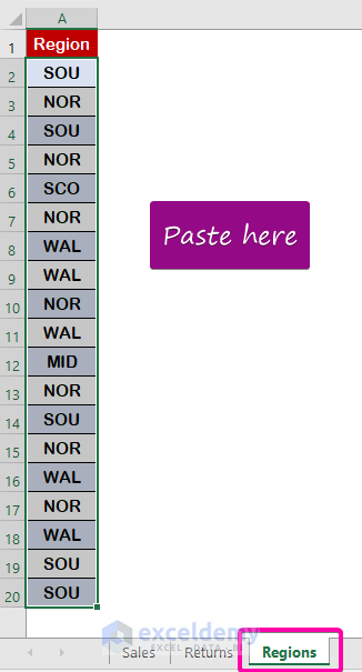
- Select the Region column and press Ctrl + C to copy.
- Go to the Regions sheet and press Ctrl + V to paste.
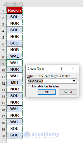
- To create a table, press Ctrl + T.
- Select the data range by enabling My table has headers.
- Click OK.
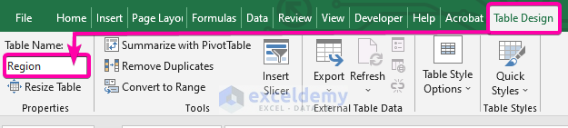
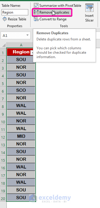
- After creating the table, name it as Region.
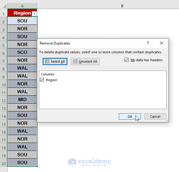
- To get the only unique values, click on the Remove Duplicates command.
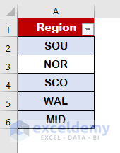
- Click OK to create the table with unique values.
- Your table for creating a slicer will be created with the unique values of different Regions.
Step 4 – Insert a PivotTable from the Sales Table
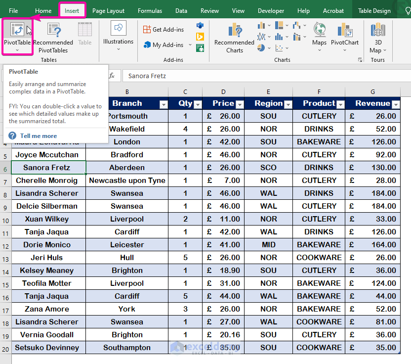
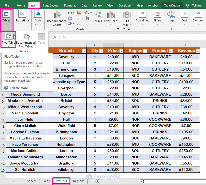
- In the Sales worksheet, click on the Insert tab.
- From the Tables ribbon, choose the PivotTable option.
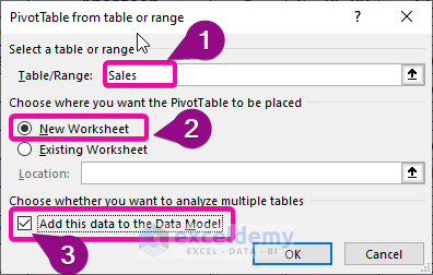
- In the Table/Range box, check whether the table name (Sales) is right.
- Click on the New Worksheet option to create the PivotTable in a new worksheet.
- Select the box Add this data to the Data Model.
- Press Enter.
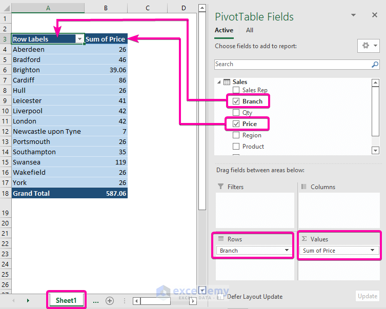
- Your first PivotTable will appear in a new worksheet (Sheet1).
- Select the fields (Branch and Price) to show in the PivotTable.
Step 5 – Insert a PivotTable with the Returns Table
- Click on the Insert tab.
- Select the PivotTable from the Tools group.
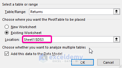
- Check the Existing Worksheet box.
- To define a location in the existing sheet, click on the right-side icon.
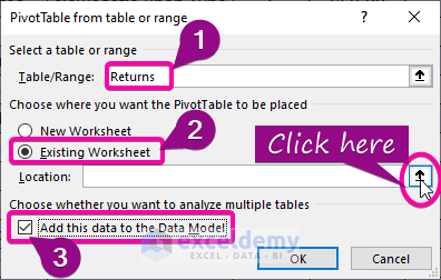
- Go to the existing PivotTable worksheet (Sheet1).
- Click on a cell (D3) to select the location for placing the new PivotTable.
- Click on the right-side icon in the box to go back.
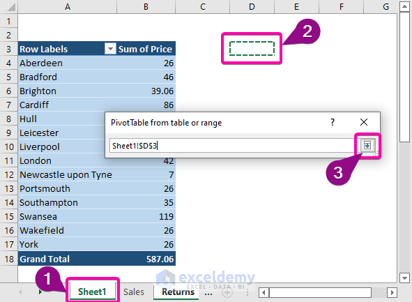
- Your selected location will appear in the Location box.
- Click Enter.
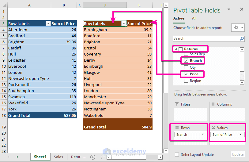
- Your second PivotTable with the Returns value will appear in the same sheet.
Step 6 – Insert a Slicer with the Region Table
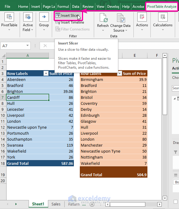
- Go to the PivotTable Analyze tab.
- From the Filter group, click on the Insert Slicer command.
- From the Slicer box, choose All.
- Click on Region.
- Press Enter.
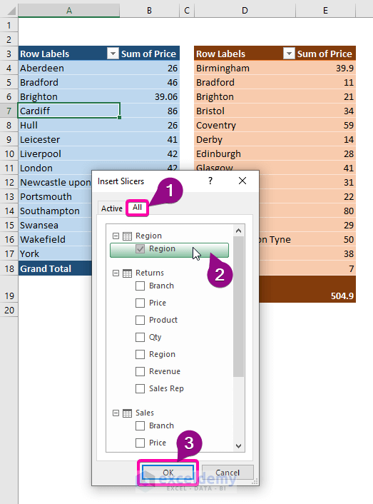
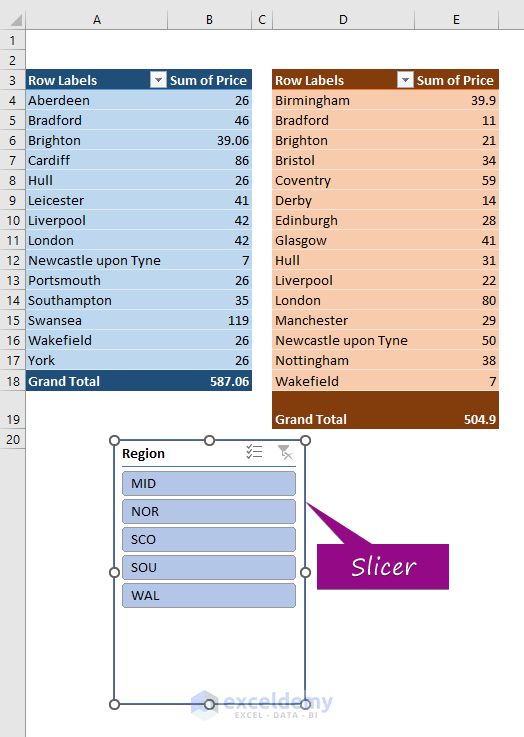
- The Slicer for the Region will show as the image shown below.
Step 7 – Build a Relationship with the Slicer
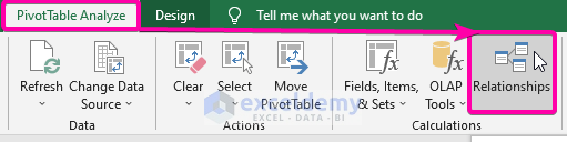
- Click on the PivotTable Analyze tab.
- From the Calculations group, click on the Relationships command.
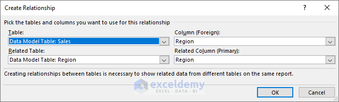
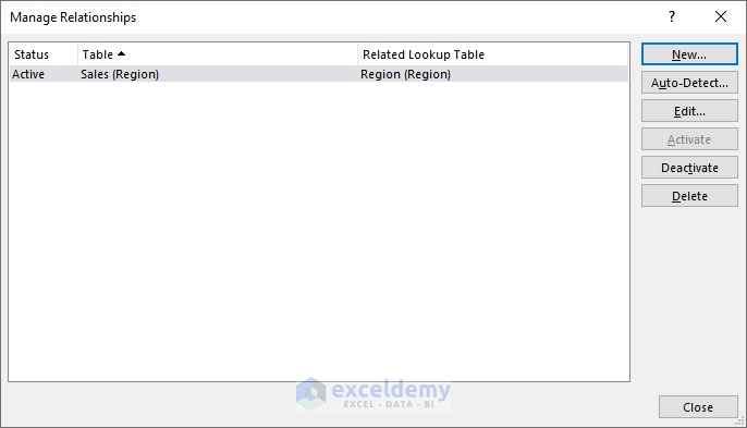
- Click on New to add the first relation.
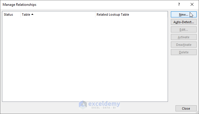
- For establishing the relation between Sales and Region, choose the following options from the drop-down lists of the Create Relationship box.
- Press Enter.
- Click again on New to create another relationship.
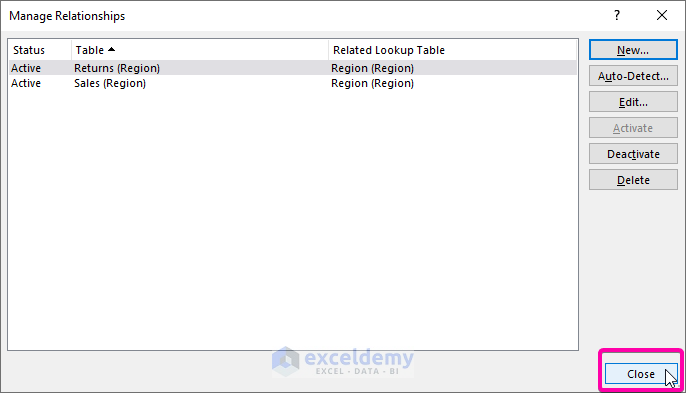
- To create the relationship between the Returns table and the Region table, select the following options as shown in the box below.

- After adding the two relationships, click on Close.
- Right-click the Slicer box.
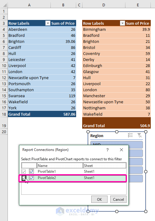
- Click on the Report Connection option from the list.
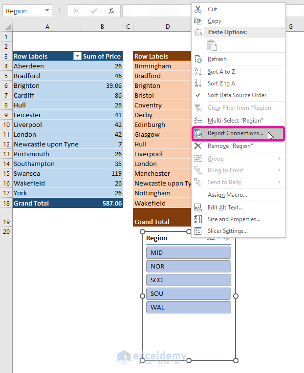
- Check both checkboxes to show the relationship between the two PivotTables.
- Click OK and your two PivotTables are connected with the Region Slicer.
Read More: Excel Slicer for Multiple Pivot Tables (Connection and Usage)
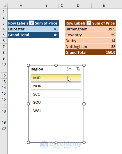
Step 8 – Final Result
- Click on a Region (such as MID), and your both PivotTables will show the relations between the Branch and Prices for the particular Region.
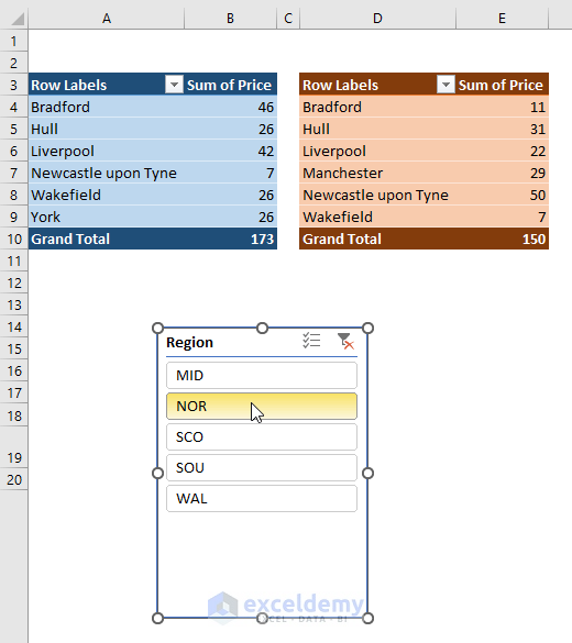
- Choose another option from the Region (NOR), and the Slicer will filter the results for both the PivotTables.
Read More: [Fixed] Report Connections Slicer Not Showing All Pivot Tables
Download the Practice Workbook
Related Articles
- How to Change Slicer Color in Excel
- How to Resize a Slicer in Excel
- How to Format Slicer in Excel
- How to Insert Slicer without Pivot Table in Excel

