How to Create an Excel Slicer with a Search Box (Easy Steps)

Excel slicers with search functionality offer a user-friendly way to filter and navigate data within Excel. By incorporating a search feature, users can quickly find and select specific items within the slicer, saving time and effort. This powerful tool enhances data analysis and decision-making by simplifying the process of filtering large datasets.

In the following, you will find an overview of Excel Slicer with a search option.

Dataset Overview

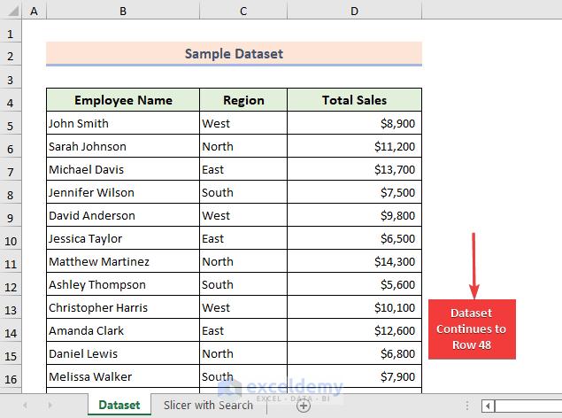
Suppose we have a dataset containing Employee Names, Regions, and Total Sales in an Excel spreadsheet. We’ll insert a slicer with a search option to filter specific items efficiently. Follow these steps:

Step 1 – Create a PivotTable

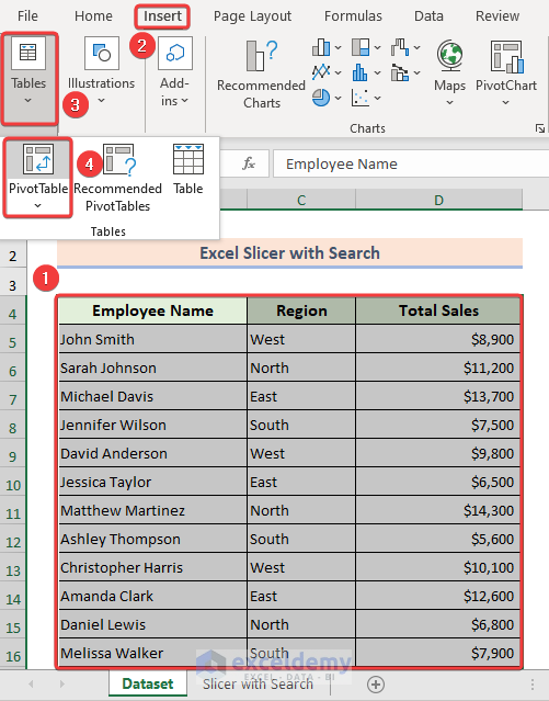
Select the entire dataset and click PivotTable from the Insert tab.

Inserting PivotTable from the insert tab

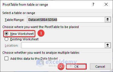
Choose New Worksheet and click OK.

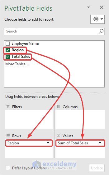
Choosing new worksheet for creating the PivotTable

From the PivotTable Fields pane, drag the Region table to the Rows section and the Total Sales table to the Values section.

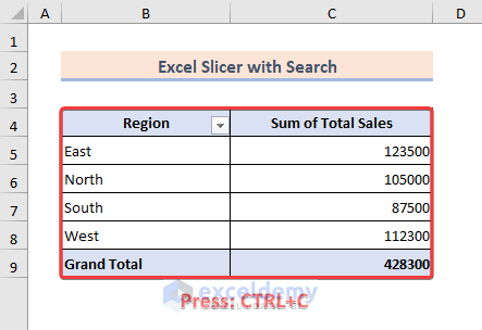
Dragging tables to multiple fields

You’ll now have a PivotTable in your worksheet. For convenience, make a copy of the PivotTable by selecting it and pressing CTRL+C to copy.

Copying the created PivotTable

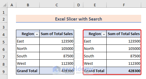
Choose a cell (E4) and paste the copied PivotTable.

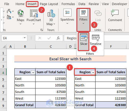
Pasting the selected PivotTable in a new location

Click any cell within the PivotTable.
Go to the Insert tab and click Slicer.

Step 2 – Insert Slicer and Check Connections

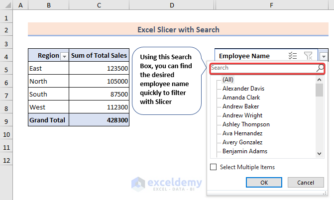
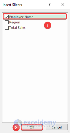
Inserting slicer from the insert tab

In the Insert Slicers window, check the box next to Employee Name and press OK.

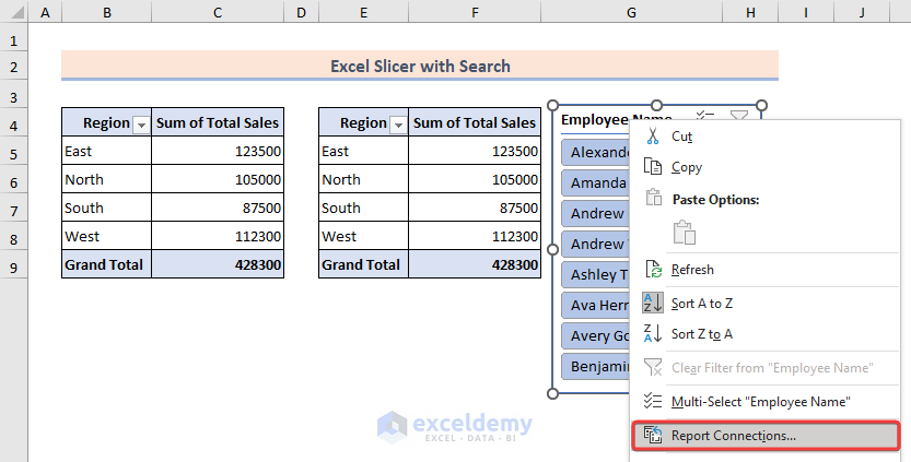
Selecting criteria for inserting a slicer

To verify that the slicer is working correctly, visit the Report Connections feature and select the slicer.

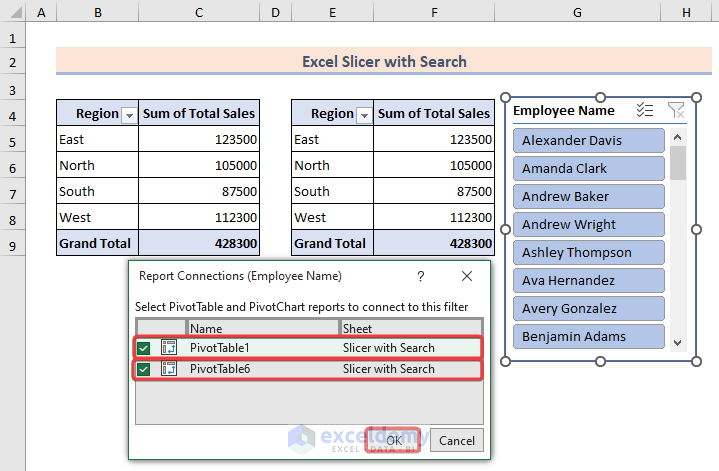
Visiting report connections options to check linking of slicer

Checkmark both the PivotTables and click OK.

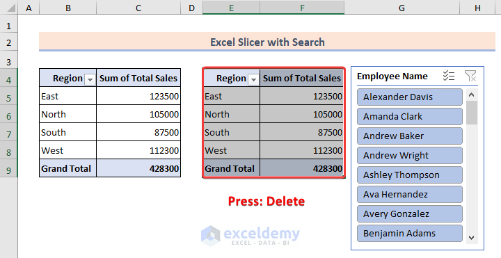
Checkmarking PivotTables to ensure connection with slicer

You can now delete the copied PivotTable (use the DELETE button on your keyboard).

Removing copied PivotTable from the worksheet

Step 3 – Add the Filter Option

Go to the Field List from the PivotTable Analyze tab.

Visiting field list from the pivottable analyze tab

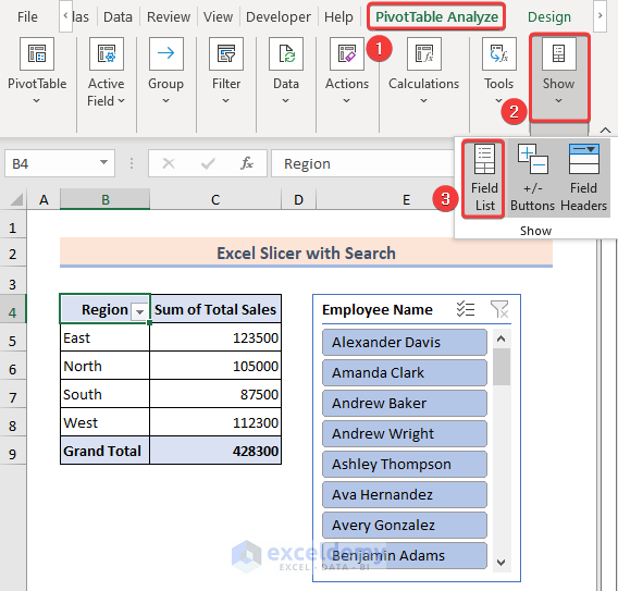
Drag the Employee Name table to the Filters section.

Dragging table to filters field

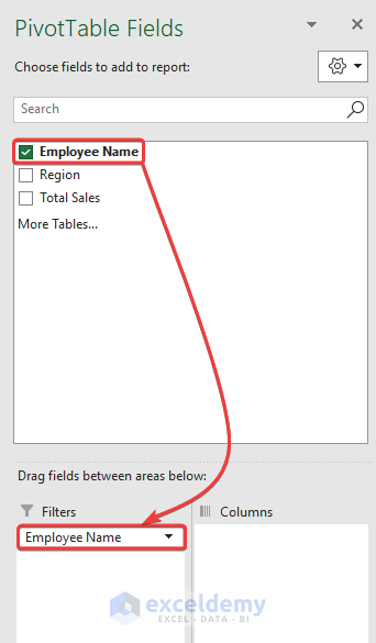
Your PivotTable now has an Employee Name filter.

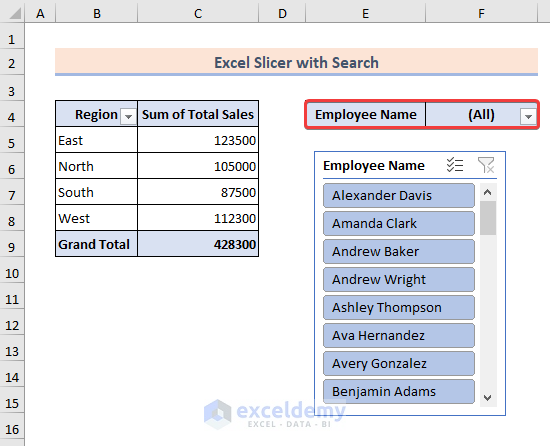
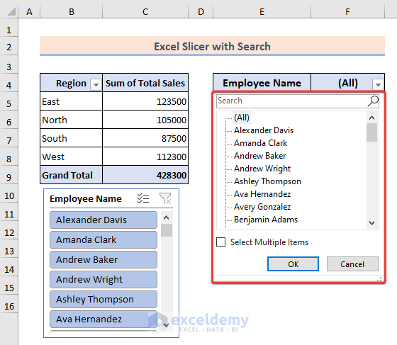
Final PivotTable for filtering tables

To check the filter, click the drop-down menu, and you’ll see all employee names listed.

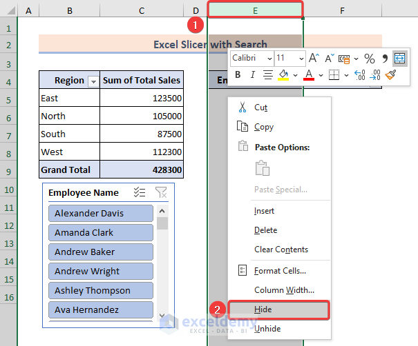
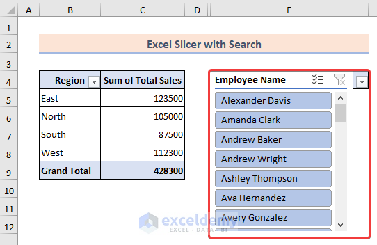
Filtering specific items from the PivotTable

Rearrange as needed (e.g., hide the column with Employee Names).

Place the slicer over the newly created filter.

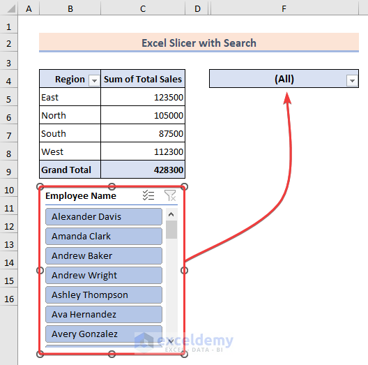
You’ve successfully created an Excel slicer with a search bar.

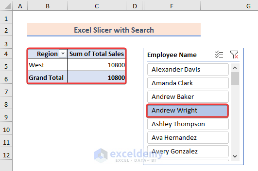
Simply click the filter icon to filter data using the slicer and choose a name from the list.

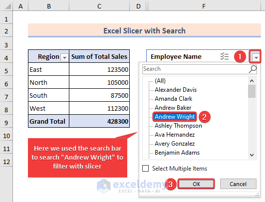
The output will display data for the selected employee name.

Final result with searching specific item from the slicer

Things to Remember

Ensure the slicer is linked to the appropriate columns or fields when creating the search option.
Choose a suitable design and layout for the slicer to avoid overlapping important data.

Frequently Asked Questions

Can I reset the slicer search and show all options again?
- Yes, you can clear the search box within the slicer to reset the search and display all available options.
Can I apply multiple search terms in Excel slicers?
- No, the search functionality in Excel slicers typically allows you to search for one term at a time.
Does the search feature in Excel slicers support wildcard characters?
- Yes, the search functionality in Excel slicers supports wildcard characters such as asterisks (*) and question marks (?).

Download Practice Workbook

You can download the practice workbook from here:

Slicer with Search.xlsx