Excel Slicer for Multiple Pivot Tables (Connection and Usage)

If you need to filter your Pivot Table too frequently, using the usual method of filtering can be time-consuming. Here comes the wonder of Slicer. It’s an array of buttons that allows filtering super fast. In this article, you will learn how to connect a slicer for multiple Pivot Tables in Excel.

What Is Slicer?

Slicer is a sophisticated way to Filter data in Excel Tables as well as Pivot Tables. It’s the quickest way to Filter out data. Other than filtering data, the slicer also shows the current state of filtering an Excel Table or a Pivot Table.

Steps to Connect Slicer for Multiple Pivot Tables in Excel

Step-1: Creating Multiple Pivot Tables to Connect Slicer

To demonstrate to you how to connect a slicer to multiple pivot tables, I will be using the following dataset as source data.

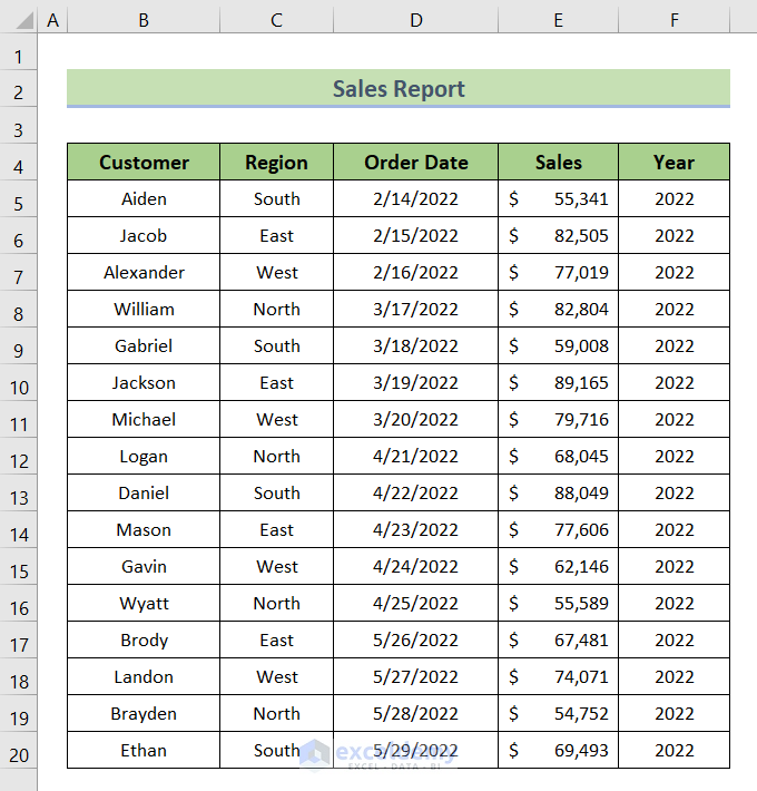
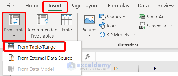
Here, I’m going to create two pivot tables for this instance. Now follow the steps below to turn the dataset above into a pivot table.

First, go to Insert ➤ PivotTable ➤ From Table/Range.

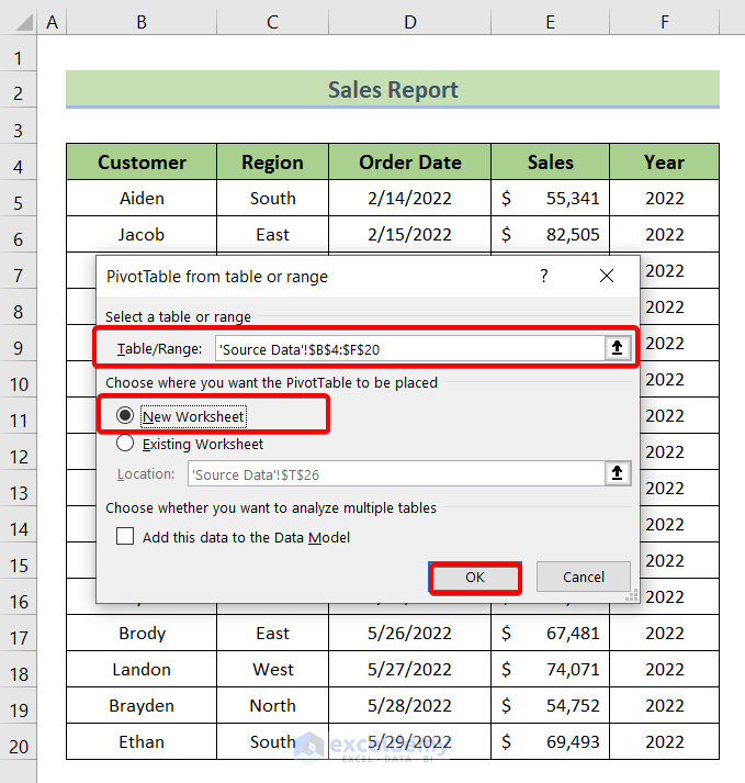
The ‘PivotTable from table or range’ dialog box will appear.

Now insert the table range in the Table/Range
Then select New Worksheet and click OK.

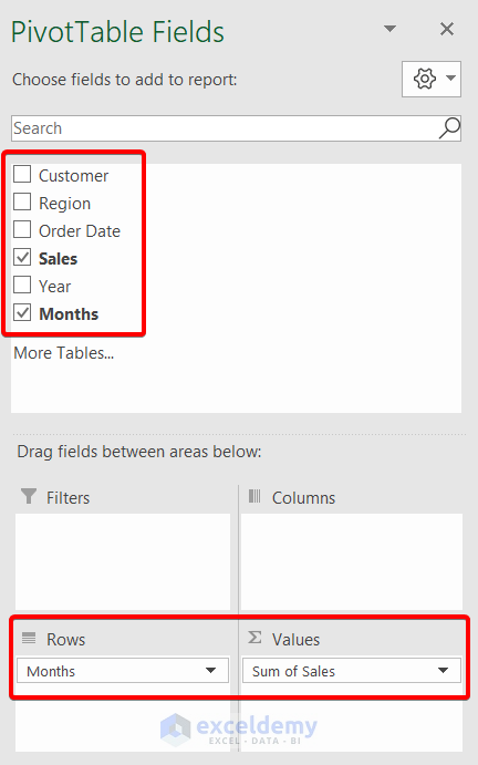
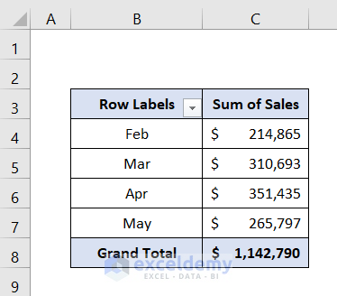
For the first Pivot Table, select the Sales and Month column in the PivotTables Field dialog box.
Then put Months under the Rows section and Sum of Sales in the Values

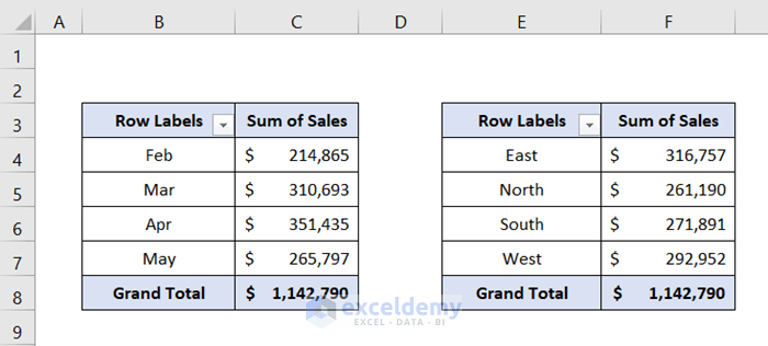
After that, you will get the first Pivot Table which has two columns.

To create the second Pivot Table,

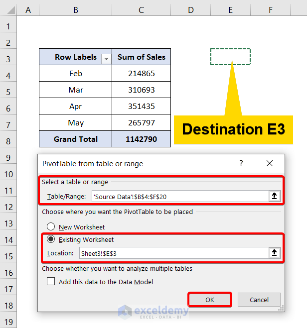
Again, go to Insert ➤ PivotTable ➤ From Table/Range.

The ‘PivotTable from table or range’ dialog box will open.

Now insert the table range again in the Table/Range
Then select Existing Worksheet.
After that pick up a cell in the Location This will be the destination of the second Pivot Table.
After that, hit OK.

This time select the Region and Sales columns in the PivotTable Fields dialog box.
Drag Region under the Rows
Under the Values section, keep the Sum of Sales.

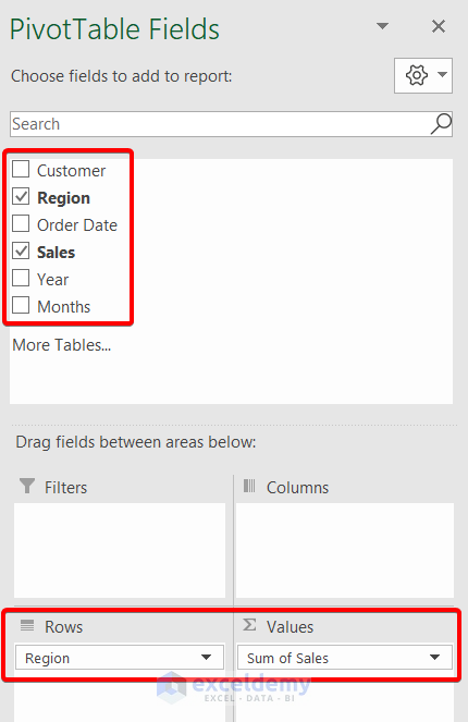
After that, you will get your second Pivot Table which has two columns.

Step-2: Inserting Slicer for Multiple Pivot Tables

Now it’s time to insert the Slicer.

To do that,

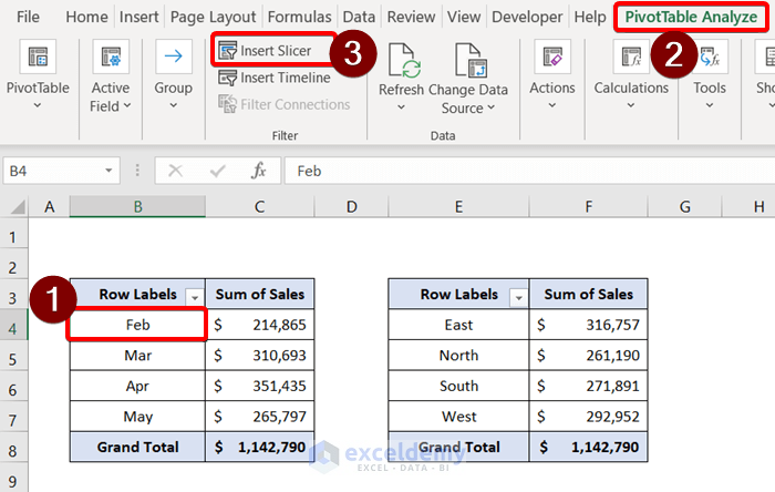
❶ Select a cell in the first Pivot Table.

❷ Then go to PivotTable Analyze ➤ Insert Slicer.

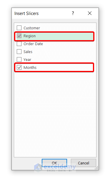
❸ Select Region and Months in the Insert Slicer dialog box.

❹ Now press OK.

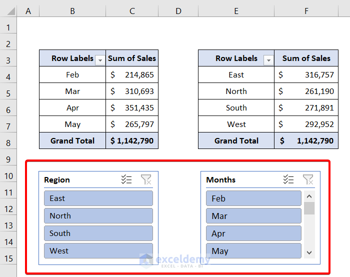
This will create two slicers named Region and Months respectively.

You can adjust the position and size of the slicers just by dragging them.

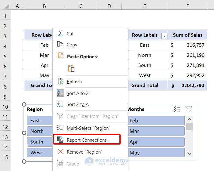
Step-3: Connecting Slicer to Multiple Pivot Tables in Excel

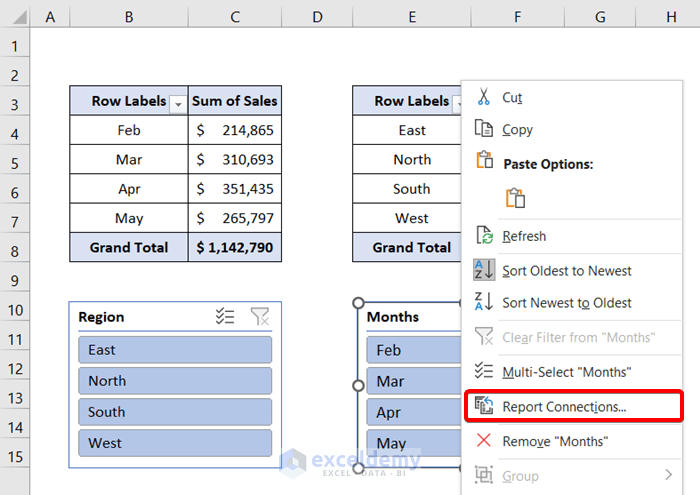
Just inserting slicers won’t work automatically. At first, you have to connect those slicers to your Pivot Tables.

To connect the Region slicer with both Pivot Tables,

❶ Right-click on the Region slicer.

❷ Then select Report Connections.

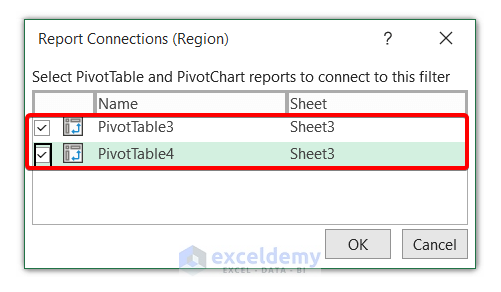
Report Connections (Region) dialog box will pop up.

❸ Check PivotTable3 and PivotTable4.

❹ Then hit OK.

So, the connection between the Region slicer and both Pivot Tables has been established.

To connect the Months slicer,

❺ Right-click on the Months slicer.

❻ Then select Report Connections.

❼ Check PivotTable3 and PivotTable4 in the Report Connections (Months) dialog box.

❽ After that, hit OK.

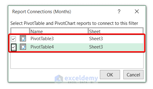
So the connection between the Months slicer and the Pivot Tables has been established.

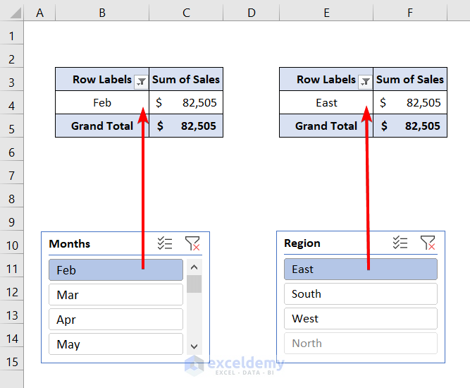
Now let’s check the slicers whether work or not.

Select Feb from the Months
Select East from the Region

As you can see, both Pivot Tables filtered data based on the selection in the slicers.

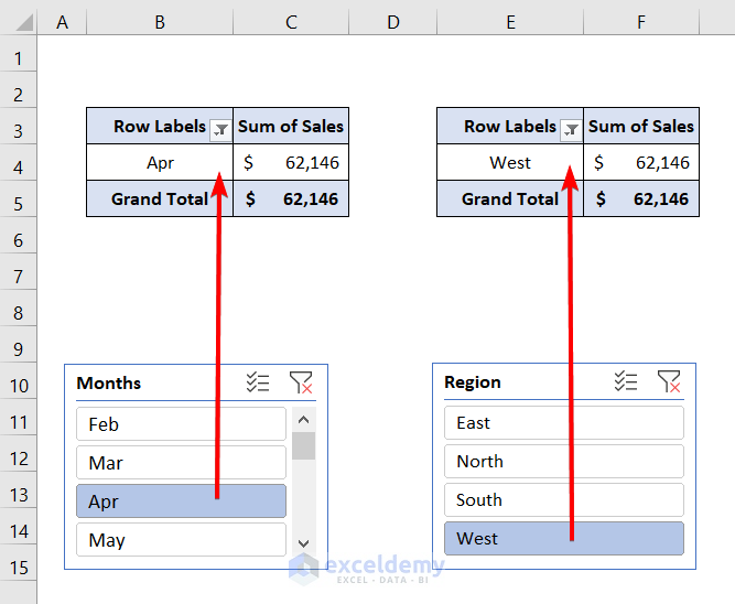
Now select Apr in the Months
Select West in the Region

As you can see, both Pivot Tables have filtered data based on the selection in the slicers.

So, this too how you can connect slicers to multiple pivot tables in Excel.

Things to Remember

Make sure you established connections between the slicers and the Pivot Tables.
Slicer is an alternative to Excel Filter.
Slicer displays the current state of the filtering.

Download Practice Workbook

You can download the Excel file from the following link and practice along with it.

Slicer for Multiple Pivot Tables.xlsx

Conclusion

To sum up, we have discussed steps to connect a slicer to multiple pivot tables in Excel. You are recommended to download the practice workbook attached to this article and practice all the methods. And don’t hesitate to ask any questions in the comment section below. We will try to respond to all the relevant queries ASAP.

<< Go Back to Pivot Table Slicer | Pivot Table in Excel | Learn Excel

Get FREE Advanced Excel Exercises with Solutions!