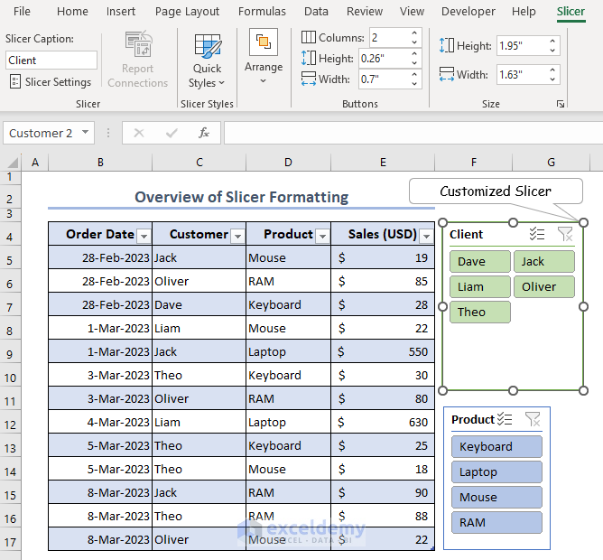
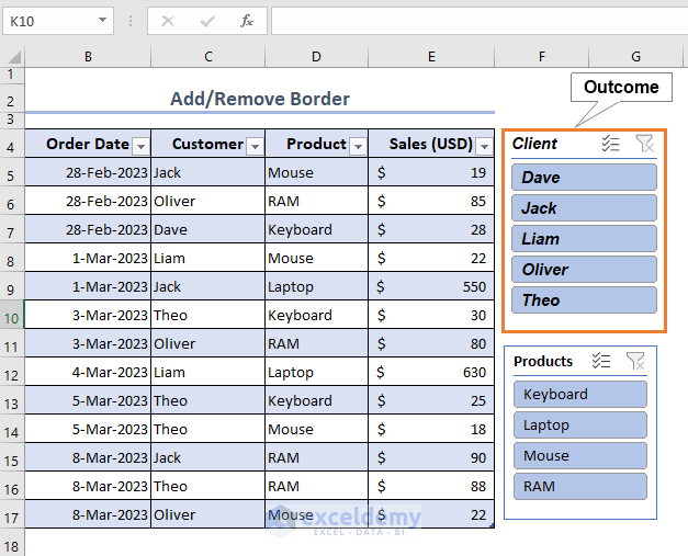
In this article, we will explain how to format the Slicer in Excel, for example by editing the size, shape, color, font, and styles, as in the image below.
What Is Slicer in Excel?
In Excel, a Slicer is a feature that allows you to filter the information you’re working with. It displays all potential values from a specified column of your data, with each value appearing as a separate button within the slicer. It is then possible to navigate the active filtering of a data set using the buttons. Users can use Slicer in Excel once they convert the dataset into an Excel Table or an Excel Pivot Table.
How to Format Slicer in Excel: 7 Common Options
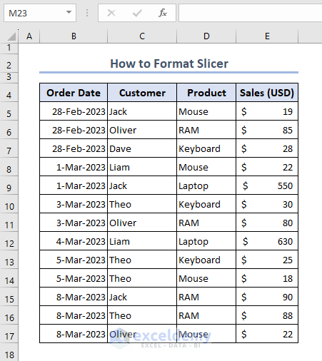
We’ll use the following dataset containing Order Date, Customer, Product, and Sales (USD) to demonstrate Slicer formatting in Excel. However, we must first convert the dataset into an Excel Table or Pivot Table in order to format the Slicer.
Option 1 – Edit or Remove Slicer Header
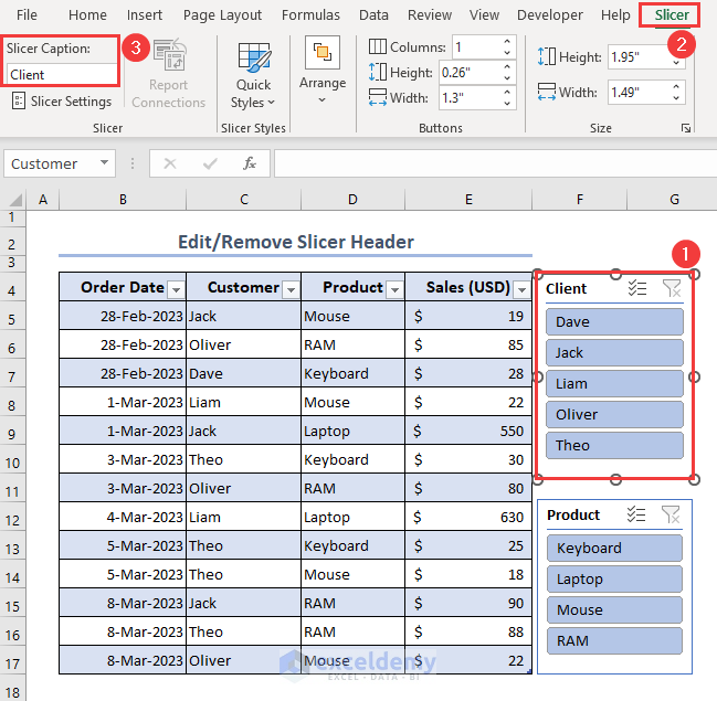
We can change, edit, or remove the Slicer header even if the Table header differs. Here, we name the Slicer header ‘Client’ whereas the Table header is ‘Customer’.
STEPS:
- Select the Slicer box.
- Go to the Slicer tab.
- Edit the Slicer Caption.
Option 2 – Change Slicer Style
STEPS:
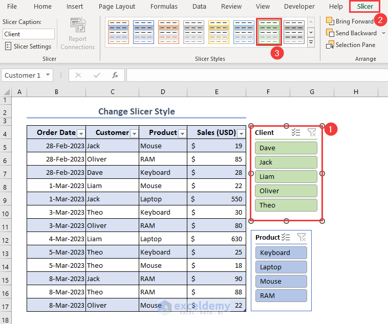
- Select the Slicer box.
- Go to the Slicer tab.
- Select the design from the Slicer Style option.
Read More: How to Change Slicer Color in Excel
Option 3 – Edit Font Size and Color
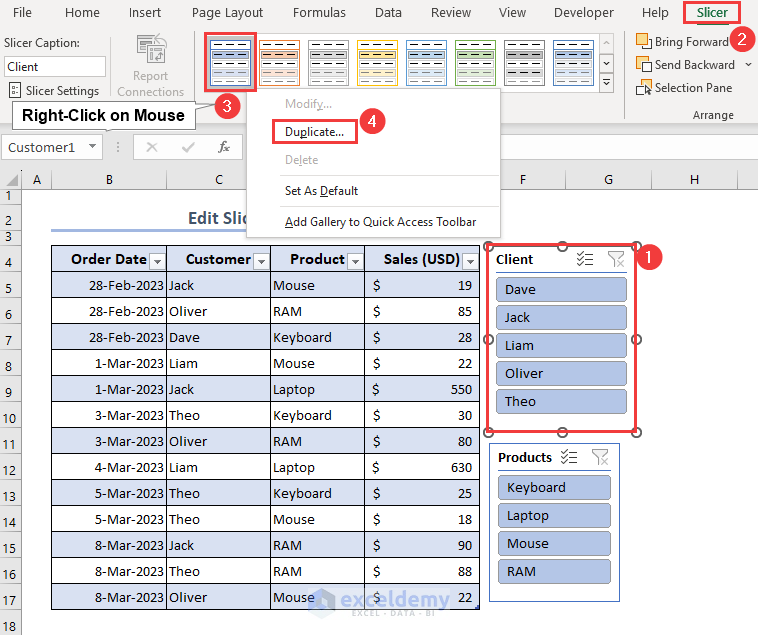
Before we can edit the font size and color of Slicer cells, we need to duplicate a style from the Slicer Style feature and modify it accordingly.
STEPS:
- Select the Slicer box.
- Go to the Slicer tab.
- Click on a design from the Slicer Style.
- Right-click on Mouse to get the Context menu.
- Select Duplicate from the Context menu.
Having created a Duplicate Slicer style, we can now change the font style.
- Rename the style from the Name field.
- Click on the Format button.
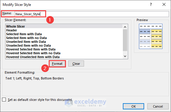
The Formal Slicer Element pop-up box appears.
- From the Font tab, select Font = Arial, and Font style = Bold Italic.
- Select Size = 11.
- Click OK.
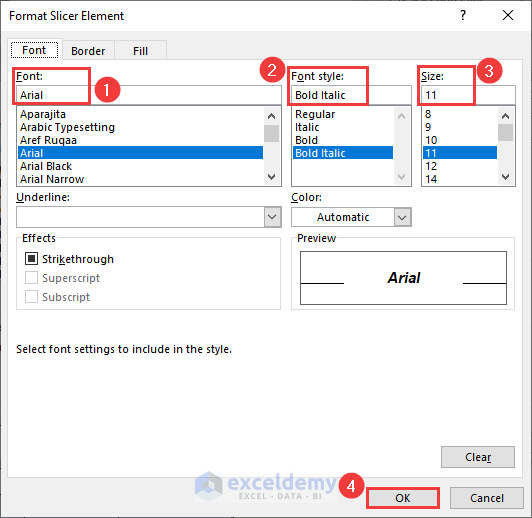
We now have Bold Italic Arial font in size 11.

Option 4 – Add or Remove Borders
STEPS:
- Go to the Border menu of the Format Slicer Element pop-up box.
- Select Line style and color presets.
- Click OK.
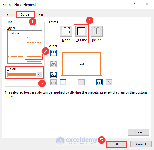
We now have an Orange color Outline border.
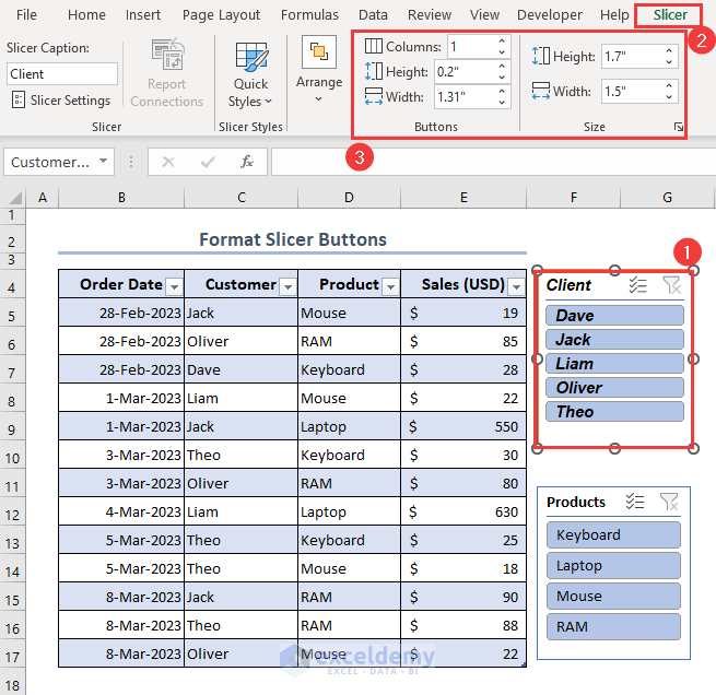
Option 5 – Format Slicer Buttons
STEPS:
- Select the Slicer box.
- Go to the Slicer tab.
- Edit from the Slicer Button and Size sections.
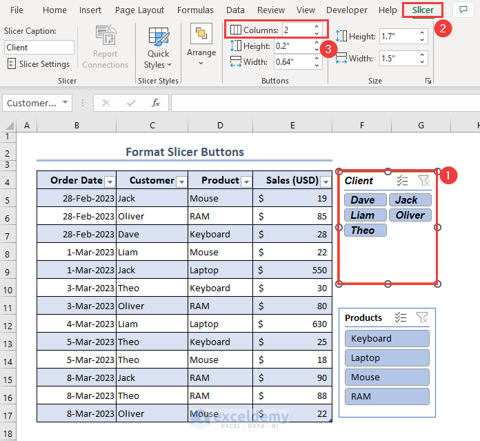
Option 6 – Multiple Columns in Slicer Box
STEPS:
- Select the Slicer box.
- Go to the Slicer tab.
- Edit the Columns field. Here, we set 2 to get 2 columns.
Read More: Excel Slicer for Multiple Pivot Tables (Connection and Usage)
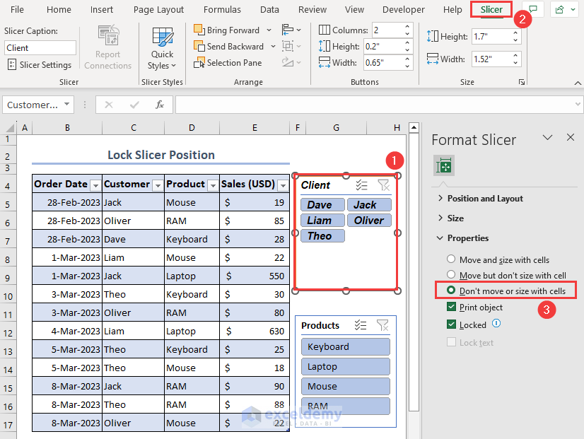
Option 7 – Lock Slicer Position
The Slicer box position changes with a change in the column width. We can easily lock the Slicer position to prevent this.
STEPS:
- Select the Slicer box.
- A pane appears on the right side.
- Select Don’t move or size with Cells rom the Properties list.
Excel Slicers Vs. Pivot Table Filters
Slicers and Pivot Table filters essentially accomplish the same thing: they reveal specific information while suppressing others. Each strategy has perks as well as drawbacks:
- The Pivot Table filters are a little clunky, whereas filtering a Pivot Table is as simple as clicking a button using Slicers.
- Filters are bound to a single Pivot Table, whereas Slicers can be linked to numerous Excel Tables, Pivot Tables, and charts.
- Filters are tied to certain rows and columns. Slicers are free-floating objects that can be moved about.
- Pivot Table filters might not function properly on touch displays. Slicers work well in many touchscreen contexts, with the exception of Excel mobile (including Android and iOS), which does not fully support this functionality.
- Slicers use considerably greater worksheet space than Pivot Table report filters.
- VBA makes it simple to automate Pivot Table filters. Automating slicers needs slightly more expertise and effort.
Frequently Asked Questions(FAQ)
1 – How do I customize my Slicer list?
Click on the Slicer box >> Go to the Slicer tab from the Top Ribbon >> Select your required design from the Slicer Styles group.
2 – How to Insert Slicer without Pivot Table?
You can insert the Slicer into an Excel Table. Select the Excel Table >> Go to the Table Design tab >> Click the Insert Slicer button.
3 – How do I change the appearance of a Slicer?
You can change the appearance of a Slicer from the Slicer Styles group. Click on the Slicer box >> Go to the Slicer tab from the Top Ribbon >> Select your required design from the Slicer Styles group.
Important Notes
- One must create an Excel Table or Pivot Table to format Slicer in Excel.
- ️ Duplication of the Slicer Style is required to modify the font and border style.
- ️ Locking the Slicer position prevents moving the Slicer with respect to column width.
Download Practice Workbook
Related Articles
- How to Resize a Slicer in Excel
- Connect Slicer to Multiple Pivot Tables from Different Data Source
- How to Insert Slicer without Pivot Table in Excel
- [Fixed] Report Connections Slicer Not Showing All Pivot Tables

