A Pivot Table is a feature in Excel that reorganizes and summarizes data from unorganized raw datasets.
In this Excel tutorial, we are going to learn how to create a pivot table with detailed steps.
The video below shows the easy steps of creating a pivot table in Excel. It shows costs and revenues of different items sold in different regions. With the help of pivot table, we organized the data to look that way instead of raw entries in rows.
In this article, we will cover
- Step-by-step approach to create a pivot table in Excel
- Creating pivot table with dates
- Method to delete a pivot table in Excel
We have used Excel for Microsoft 365 for this demonstration. However, the pivot table feature is available to all versions of Excel.
What Is a Pivot Table in Excel?
A Pivot Table in Excel is a powerful tool that can help you summarize and analyze large amounts of data. It can help you to generate insights into large datasets quickly. Also, you can sort, filter, and calculate data in a more digestible way.
You can quickly categorize and analyze data using a Pivot Table based on several criteria, including dates, categories, and other elements. You can add, count, average, and discover the maximum and minimum values among other calculations.
What Is a Pivot Table Used for in Excel?
The main purpose of a Pivot Table is to summarize and analyze large amounts of data in an organized way. Here, we can list some of the common uses of pivot tables in Excel below:
- Data Summarization
- Data Comparison
- Data Analysis
- Data Visualization
In practical life, you can compare the total sales of different products, show sales of different products as a percentage of grand total, combine duplicate data, count employee numbers for different departments, insert values to empty rows, and many more.
How to Create a Pivot Table in Excel: 7 Easy Steps
To create a Pivot Table in Excel, we are using a dataset that contains the cost and revenue of different products in different regions. We will generate a region-wise summary of the cost and revenue for the products using a Pivot Table in Excel.
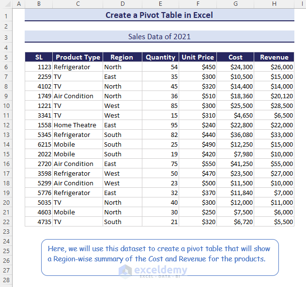
The following steps will guide you on how to create a Pivot Table in Excel.
Step-01: Inserting Pivot Table in Excel
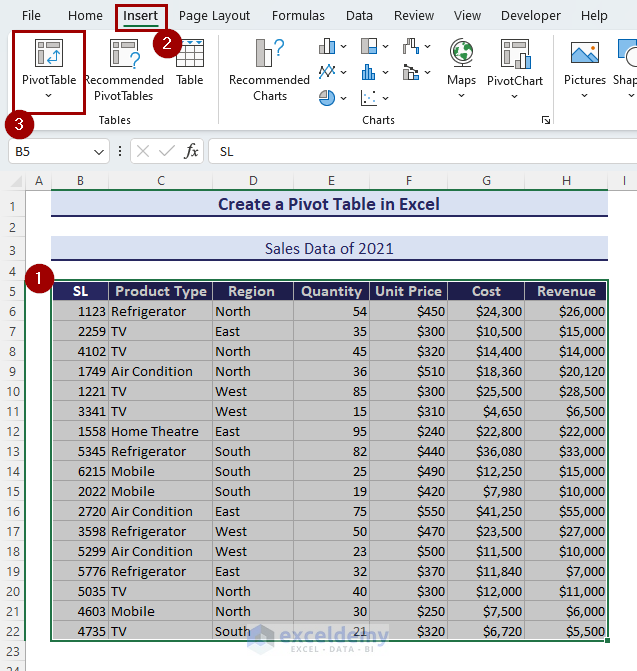
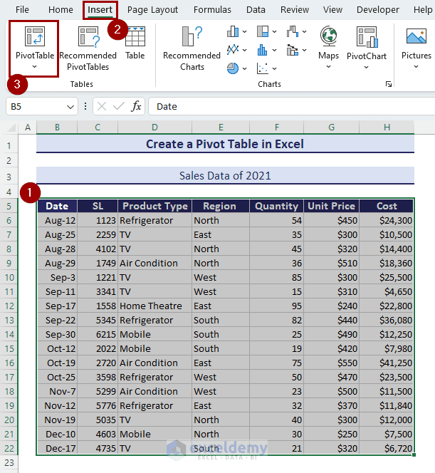
First of all, you need to insert a Pivot Table in Excel.
- To insert a Pivot Table, select the data range (B4:H21) ➤ Insert ➤ PivotTable.
- As a result, a dialog box named Create PivotTable will appear.
- Select New Worksheet ➤ OK in the Create PivotTable dialog box.
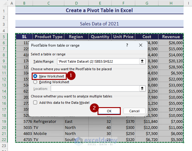
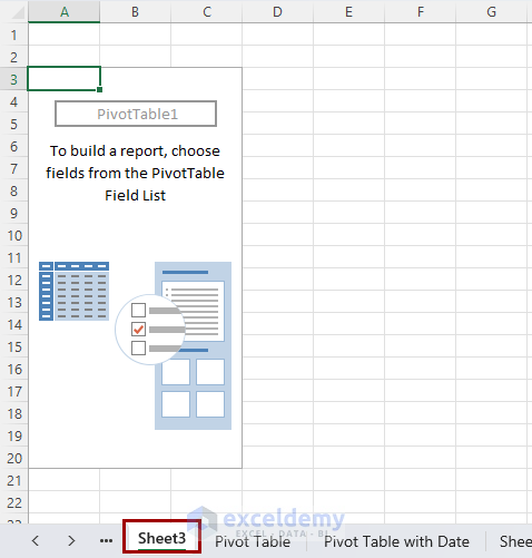
- A Pivot Table will be inserted into a new worksheet.
Read More: How to Insert Pivot Table in Excel
What to Do to Insert Pivot Table in the Existing Sheet?
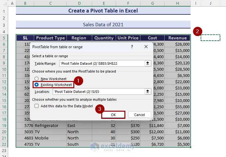
- To insert a Pivot Table in the existing sheet, select the data range (B4:H21) ➤ Insert ➤ PivotTable.
- Now, in the Create PivotTable box, select Existing Worksheet.
- After that, select the cell where you want to place the Pivot Table.
- Then, click OK.
There’s another way of inserting a Pivot Table in the same worksheet.
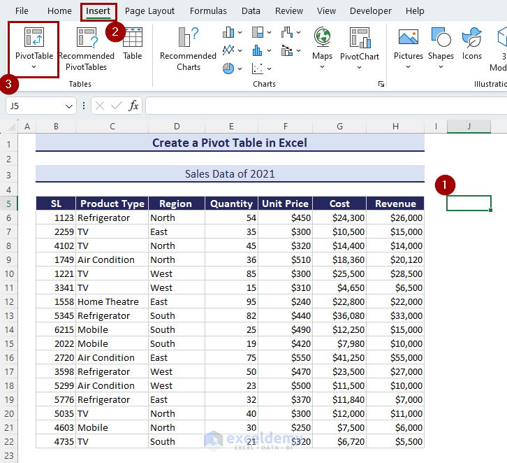
- To insert a Pivot Table in the same worksheet, select a cell outside the data range (B4:H21) ➤ Insert ➤ PivotTable.
- In the Create PivotTable box, click on the marked icon.
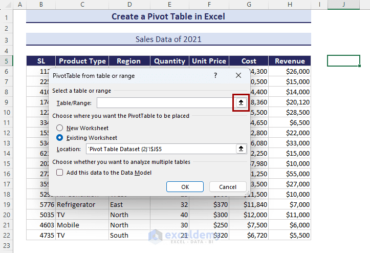
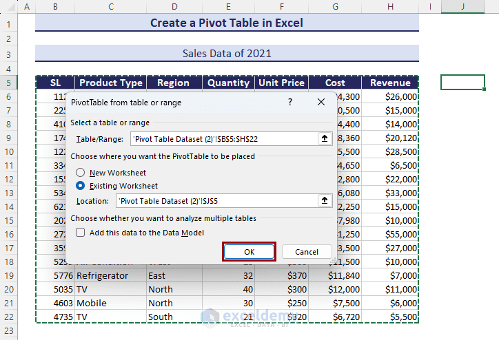
- After that, select the table or range you want to use for creating the Pivot Table.
- Then, click OK to see the Pivot Table in the existing sheet.
Step-02: Adding Fields to Pivot Table
In this step, I will show you how to add fields to the Pivot Table. Here, I will work on the PivotTable Fields task pane to lay out the Pivot Table.
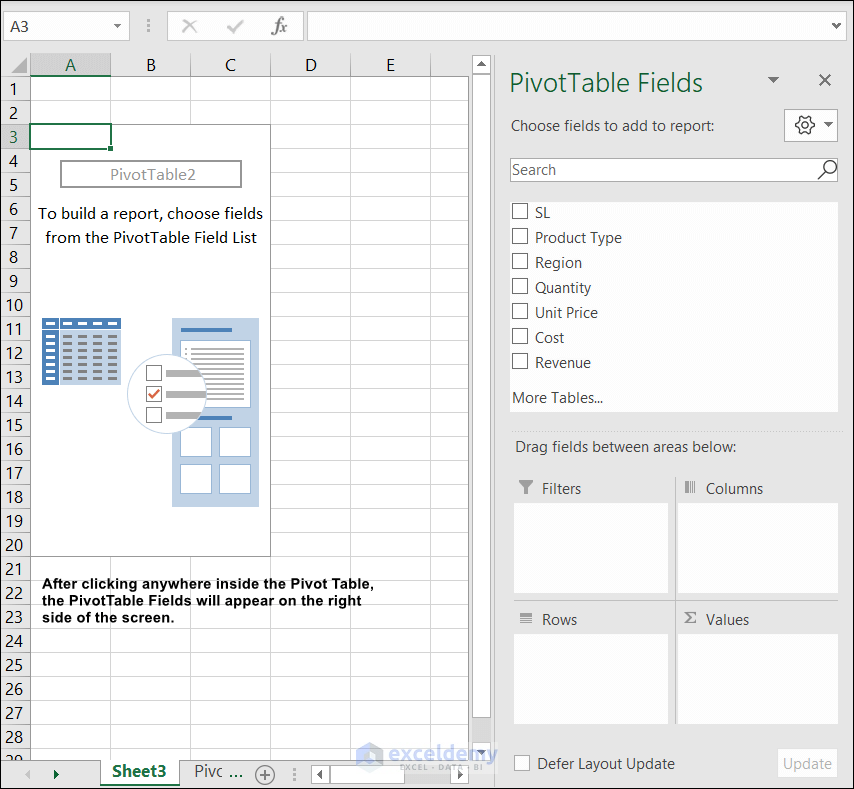
After inserting Pivot Table, the PivotTable Fields will appear on the right side of the screen. The PivotTable Fields task pane has two parts: the upper part, where the field names reside, and the lower part, where you will place the field names from the upper part.
You can lay out the Pivot Table in the following ways:
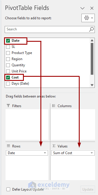
- Firstly, select and drag the field names (at the top of the PivotTable Fields task pane) to one of the four boxes at the bottom of the task pane.
- Here, I dragged the Cost and Revenue fields into the Values The Pivot Table will display the total of all the values in the Sum of Cost and Sum of Revenue columns respectively.
- Secondly, select and drag the field names you want in your Row Labels into the Rows section.
- Here, I selected the Region and Product Type fields in the Rows section.
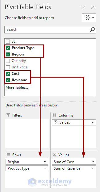
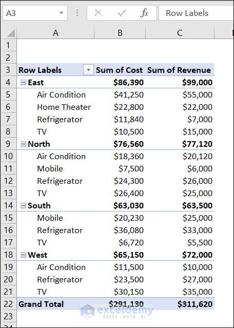
- The following figure gives me the desired Pivot Table.
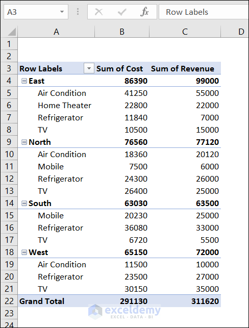
- From this Pivot Table, you can easily find out the Grand Total of the region-wise Cost and Revenue for different products.
The pivot table usually shows the sum values of numbers. We can also change them to other summaries using the following steps.
- Right-click on a value field cell and select Value Field Settings from the context menu.
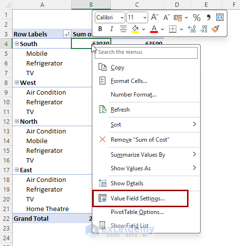
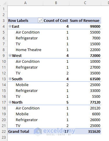
- Select the summary you prefer from the Summarize value field by We have chosen Count here.
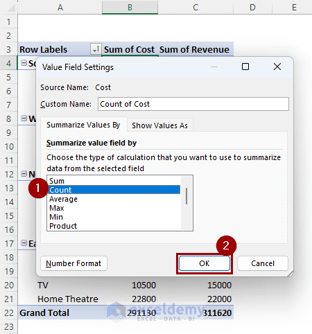
- Clicking on OK will change the summary calculation.
Read More: How to Create Pivot Table Report in Excel
Step-03: Formatting Numbers in Pivot Table in Excel
In this step, I will explain how you can change the Number Format in the Pivot Table.
- First of all, right-click on any cell of the Pivot Table where you want to change the Number Format.
- Secondly, select Number Format.
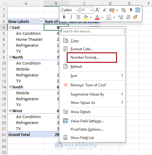
- After that, a dialog box named Format Cells will appear.
- Select the Category you want. Here, I selected Currency.
- Then, click OK.
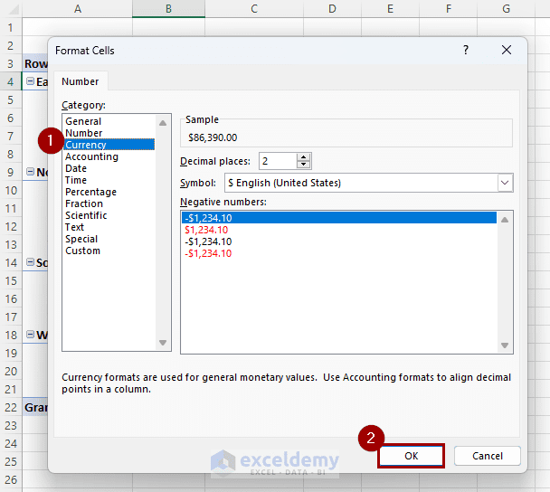
- In the following picture, you can see that the Number Format has changed to Currency.
Step-04: Refreshing Values in Pivot Table
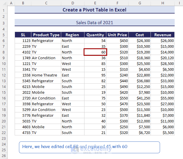
Pivot Table does not automatically update when you edit or make a change in the main dataset. To update a Pivot Table, you need to refresh it.
We have used the dataset below to create the Pivot Table. In the dataset, we have changed the value of Cell E7 from 45 to 60.
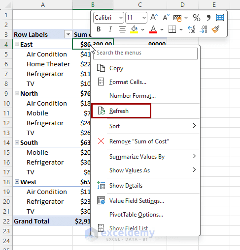
- To update the Pivot Table, right-click on any cell of the Pivot Table and select Refresh.
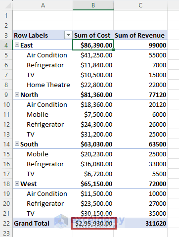
- As a result, the data in the Pivot Table will be updated.
Read More: VBA to Create Pivot Table
Step-05: Sorting Data in Pivot Table
In this fifth step, I will show you how you can sort data in a Pivot Table.
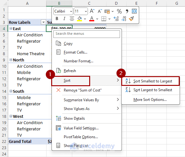
- Firstly, right-click on any cell from the column where you want to sort data.
- Then, select Sort and choose the sorting order you want.
- Here, I selected Sort Smallest to Largest.
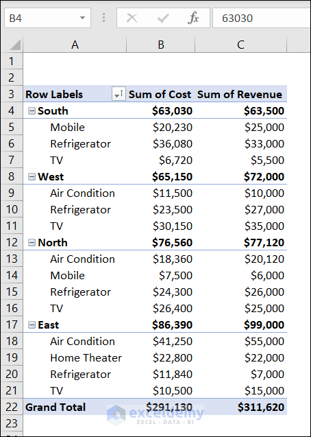
- As a result, the data in the Sum of Cost column inside the Pivot Table will be sorted in the order you selected.
Step-06: Adding Percent of Total in Pivot Table
Here, I will explain how to add Percent of Grand Total in your Pivot Table.
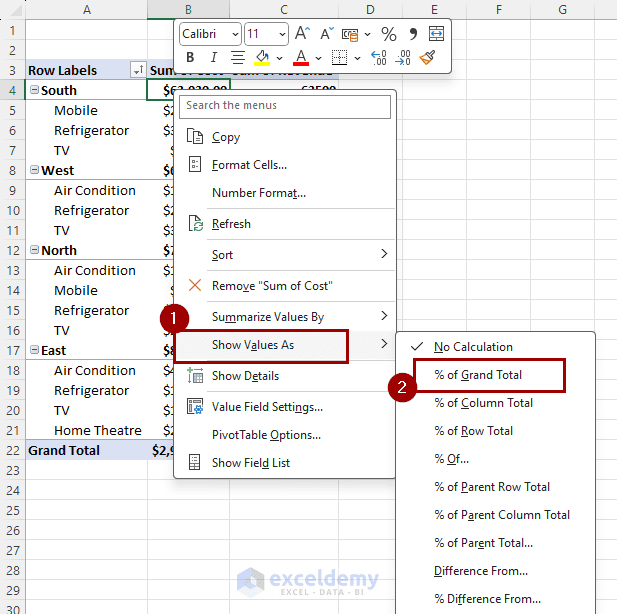
- Select any cell where you want to add a Percent of Grand Total.
- Then, select Show Values As ➤ % of Grand Total.
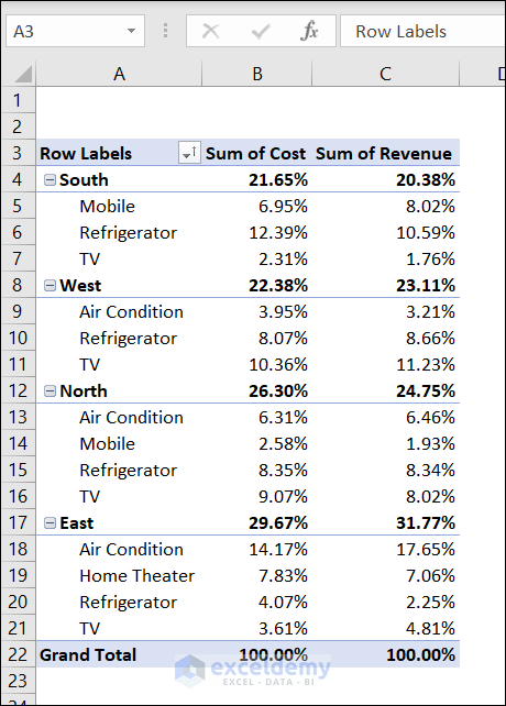
- In the following picture, you can see that Percent of the Grand Total is added to the Pivot Table.
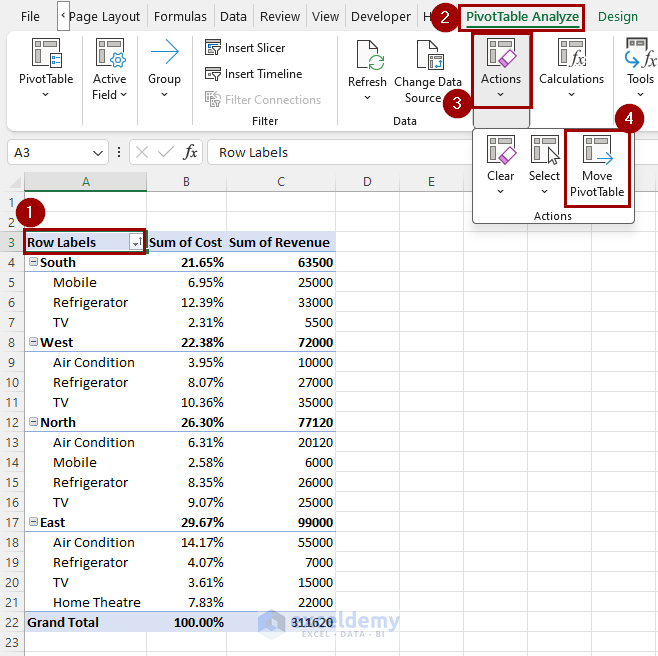
Step-07: Moving Pivot Table to a New Location in Excel
In this step, I will show you how you can move the Pivot Table in Excel to a new location.
- To do so, select any cell of the Pivot Table ➤ PivotTable Analyze ➤ Actions ➤ Move PivotTable.
- A Move PivotTable dialog box will appear.
- Select the Location where you want to move the Pivot Table and click on OK.
- Here, I selected Cell D3 in the Existing Worksheet.
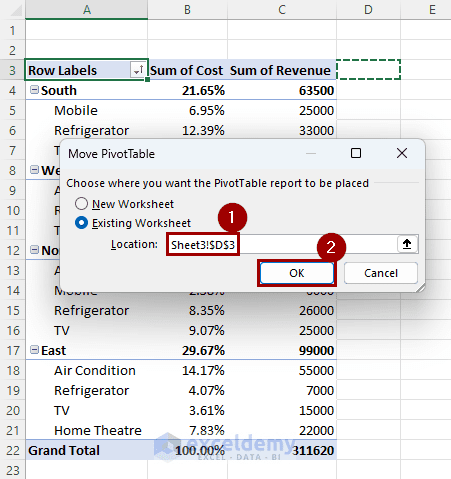
- After selecting OK, the Pivot Table will be moved to the desired location.

How to Create a Pivot Table in Excel with Dates
In this section, I will explain how to create a Pivot Table in Excel with dates. The dataset contains the dates on which the products were sold. We will try to find the date-wise and month-wise cost of the products. Let’s see the steps.
- To insert a pivot table with dates, select the data range (B4:H21) ➤ Insert ➤ PivotTable.
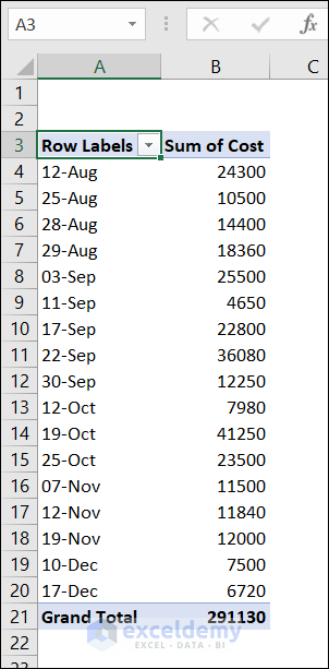
- Drag Cost in the Values section and Date in the Rows section.
- As a result, you will see the date-wise Sum of Cost in the Pivot Table.
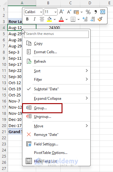
- To see the month-wise sum of cost, right-click on any cell inside the Pivot Table and select Group from the drop-down menu.
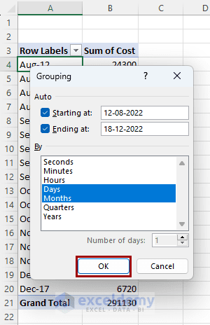
- After that, select Months in the Grouping box and click OK.
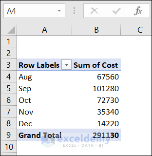
- As a result, you will see the month-wise sum of the cost of the products.
How to Delete a Pivot Table in Excel
To delete a Pivot Table, you can follow the steps below.
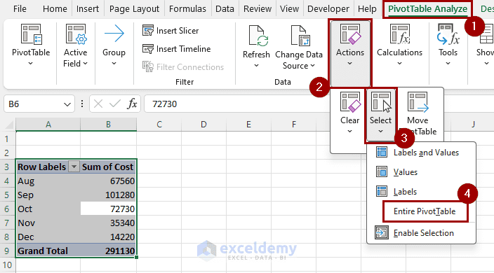
- Select any cell inside the Pivot Table.
- After that, select PivotTable Analyze ➤ Select ➤ Entire PivotTable.
- Next, click on the Delete key on the keyboard.
Things to Remember
You must remember that if you group any date in your Pivot Table it will be grouped in all the other worksheets of that workbook.
Download Practice Workbook
You can download the practice workbook from here.
Conclusion
In this article, I explained how to create a Pivot Table in Excel. Here, I explained it in easy steps. I hope this article was clear to you.
Create a Pivot Table in Excel: Knowledge Hub
- How to Automatically Create Pivot Table in Excel
- How to Create Pivot Table in Excel for Different Worksheets
- How Do I Create a Pivot Table from Multiple Worksheets
- VBA Code to Create Pivot Table with Dynamic Range
- Use of VBA to Create Pivot Table from Named Range
<< Go Back to Pivot Table in Excel | Learn Excel
Get FREE Advanced Excel Exercises with Solutions!

Hi, what an excellent article series!
Straight and to the point, very easy to follow, practice and understand.
Many thanks!
P.S. Why does Excel 2016 show “security warning – external data connection” after downloading the example Excel files?