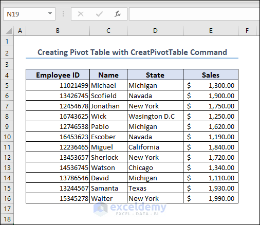
Method 1 – Inserting a Pivot Table with CreatePivotTable Command
Steps:
- Create a dataset to insert the pivot table. Check out our dataset for representation.
- Insert a new module in the VBA window.
- Enter the following code into the module:
Code:
Sub CreatePivotTable()
    Dim ws As Worksheet
    Dim outputWs As Worksheet
    Dim pvt As pivotTable
    Dim pvtCache As pivotCache
    ' Set the worksheet where the pivot table will be created
    Set ws = ThisWorkbook.Worksheets("CreatePivotTable")
    ' Set the output worksheet where the pivot table will be placed
    Set outputWs = ThisWorkbook.Worksheets("CreatePivotTable_Output")
    ' Set the range of data that will be used to create the pivot table
    Set pvtCache = ThisWorkbook.PivotCaches.Create(SourceType:=xlDatabase, SourceData:=ws.Range("B4:E16"))
    ' Create the pivot table using the pivot cache
    Set pvt = pvtCache.CreatePivotTable(TableDestination:=outputWs.Range("B4"))
    ' Set the row and column fields, as well as the values for the pivot table
    With pvt
        .PivotFields("State").Orientation = xlRowField
        .PivotFields("Employee ID").Orientation = xlRowField
        .AddDataField .PivotFields("Sales"), "Total Sales", xlSum
    End With
End Sub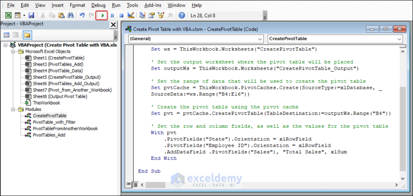
- Run the code.
Code Breakdown:
- The code starts by declaring variables for worksheets, pivot table, and pivot cache.
- It sets the “ws” variable to represent the worksheet where the pivot table will be created, which is named “CreatePivotTable“.
- It sets the “outputWs” variable to represent the output worksheet where the pivot table will be placed, which is named “CreatePivotTable_Output“.
- The pivot cache is created using the “Create” method of the PivotCaches object. It specifies the data source as the range “B4:E16” on the “ws” worksheet.
- The pivot table is created using the “CreatePivotTable” method of the pivot cache. It specifies the destination range as the “B4” cell on the “outputWs” worksheet.
- The row and column fields of the pivot table are set using the “Orientation” property of the PivotFields object. In this code, the “State” field is set as a row field, and the “Employee ID” field is set as a row field.
- The data field is added to the pivot table using the “AddDataField” method of the pivot table’s PivotFields object. It specifies the “Sales” field to be summed and assigns it the name “Total Sales“.
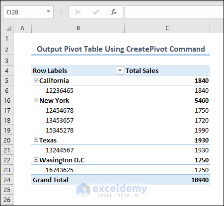
- Finally, you will see an output like the given image in your worksheet.
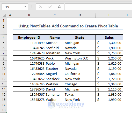
Method 2 – Using Pivot Tables: Adding a Command for Making a Pivot Table
Steps:
- Prepare a dataset. Check out our dataset for representation.
- Insert a new module in the VBA window.
- Enter the following code into the module and run it.
Code:
Sub PivotTables_Add()
    Dim ws As Worksheet
    Dim outputWs As Worksheet
    Dim pvt As pivotTable
    Dim pvtCache As pivotCache
    Dim dataRange As Range
    Dim pvtRange As Range
    ' Set the worksheet where the pivot table will be created
    Set ws = ThisWorkbook.Worksheets("PivotTables_Add")
    ' Set the output worksheet where the pivot table will be placed
    Set outputWs = ThisWorkbook.Worksheets("PivotTables_Add_Output")
    ' Set the range of data that will be used to create the pivot table
    Set dataRange = ws.Range("B4:E16")
    ' Set the range where the pivot table will be placed
    Set pvtRange = outputWs.Range("B4")
    ' Create a pivot cache based on the data range
    Set pvtCache = ThisWorkbook.PivotCaches.Create(SourceType:=xlDatabase, SourceData:=dataRange)
    ' Create a pivot table using the pivot cache
    Set pvt = outputWs.PivotTables.Add(pvtCache, pvtRange, "MyPivotTable")
    ' Set the row and column fields, as well as the values for the pivot table
    With pvt
        .PivotFields("State").Orientation = xlRowField
        .PivotFields("Employee ID").Orientation = xlRowField
        .AddDataField .PivotFields("Sales"), "Total Sales", xlSum
    End With
End Sub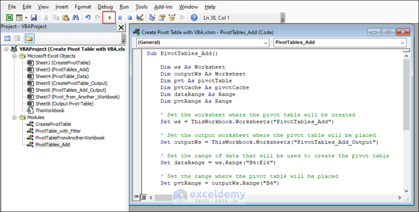
Code Breakdown:
- The code starts by declaring variables for worksheets, pivot table, pivot cache, data range, and pivot table range.
- It sets the “ws” variable to represent the worksheet where we will create the pivot table, which we named as “PivotTables_Add“.
- It sets the “outputWs” variable to represent the output worksheet where we will place the pivot table, which we named as “PivotTables_Add_Output“.
- We defined the data range using the “Range” method on the “ws” worksheet. In this code, we set the data range as “B4:E16“.
- We defined the pivot table range using the “Range” method on the “outputWs” worksheet. This code sets the pivot table range as “B4“.
- Then, we created a pivot cache using the “Create” method of the PivotCaches object. It specifies the data source as the “dataRange“.
- We also created the pivot table using the “Add” method of the PivotTables object on the “outputWs” worksheet. It specifies the pivot cache pivot table range and assigns the name “MyPivotTable” to the pivot table.
- We set the row and column fields of the pivot table using the “Orientation” property of the PivotFields object. In this code, the “State” field is set as a row field, and the “Employee ID” field is set as a row field.
- The data field is added to the pivot table using the “AddDataField” method of the pivot table’s PivotFields object. It specifies the “Sales” field to be summed and assigns it the name “Total Sales“.
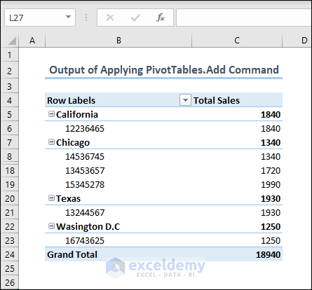
- After running the code, you will see the pivot table in your workbook.
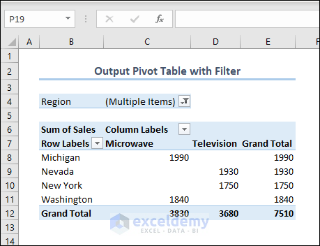
Method 3 – Inserting a Pivot Table with Filter Using VBA in Excel
Steps:
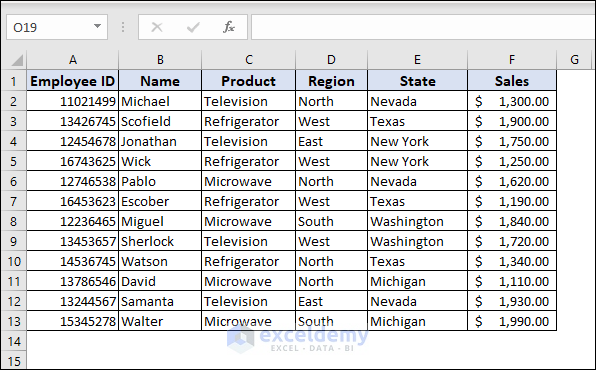
- Create a dataset. Here, we added two more columns: ‘Region’ and ‘Product’ to show filtering.
- Insert a new module in the VBA window.
- Enter the following code into the module and Run it.
Code:
Sub PivotTable_with_Filter()
Dim PV_Sheet As Worksheet, DS_Sheet As Worksheet
Dim PV_Cache As pivotCache
Dim PV_Table As pivotTable
Dim PV_Range As Range
Dim LtRow As Long, LtColumn As Long
Dim xSheet1 As Variant
On Error Resume Next
With Application
.DisplayAlerts = False
.ScreenUpdating = False
End With
For Each xSheet1 In ActiveWorkbook.Worksheets
If xSheet1.Name = "Output Pivot Table" Then
xSheet1.Delete
End If
Next xSheet1
Worksheets.Add.Name = "Output Pivot Table"
Set PV_Sheet = Worksheets("Output Pivot Table")
Set DS_Sheet = Worksheets("PivotTable_Data")
LtRow = DS_Sheet.Cells(Rows.Count, 1).End(xlUp).Row
LtColumn = DS_Sheet.Cells(1, Columns.Count).End(xlToLeft).Column
Set PV_Range = DS_Sheet.Cells(1, 1).Resize(LtRow, LtColumn)
Set PV_Cache = ActiveWorkbook.PivotCaches.Create(SourceType:=xlDatabase, SourceData:=PV_Range).CreatePivotTable(TableDestination:=PV_Sheet.Cells(2, 2), TableName:="Automatically Created PivotTable")
Set PV_Table = PV_Cache.CreatePivotTable(TableDestination:=PV_Sheet.Cells(1, 1), TableName:="Automatically Created PivotTable")
With ActiveSheet.PivotTables("Automatically Created PivotTable").PivotFields("Region")
.Orientation = xlPageField
End With
With ActiveSheet.PivotTables("Automatically Created PivotTable").PivotFields("State")
.Orientation = xlRowField
End With
With ActiveSheet.PivotTables("Automatically Created PivotTable").PivotFields("Product")
.Orientation = xlColumnField
End With
With ActiveSheet.PivotTables("Automatically Created PivotTable").PivotFields("Sales")
.Orientation = xlDataField
.Function = xlSum
End With
End Sub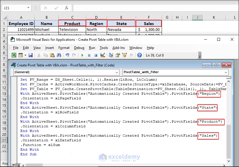
Code Breakdown:
- The code begins by declaring variables for worksheets, pivot cache, pivot table, and range.
- It turns off display alerts and screen updating for improved performance.
- It checks if a worksheet named “Output Pivot Table” already exists and deletes it if found.
- It adds a new worksheet named “Output Pivot Table” to store the pivot table.
- We assigned the PV_Sheet and DS_Sheet variables references to the “Output Pivot Table” worksheet and the “PivotTable_Data” worksheet, respectively.
- Then, we used the LtRow and LtColumn variables to determine the last row and last column of data in the DS_Sheet.
- We set the PV_Range variable to the range of data in the DS_Sheet using the Resize method.
- We created the PV_Cache by specifying the data source range PV_Range.
- Finally, we created the PV_Table using the PV_Cache and positioned it at cell B2 of the PV_Sheet.
- The pivot table fields are configured:
- We set the “Region” field as a page field, the “State” field as a row field, the “Product” field as a column field, and the “Sales” field as a data field with the “Sum” function applied.
- Afterward, you will see a pivot table with a filter in your workbook.
How to Create a Pivot Table from Another Workbook Using Excel VBA
Steps:
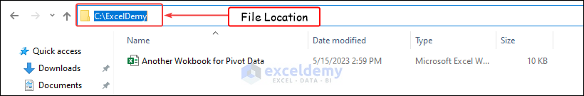
- Check out the Excel file location from which you want to create the pivot table.
- Use the directory for the code. Our file directory is “C:\ExcelDemy\Another Wokbook for Pivot Data.xlsx”
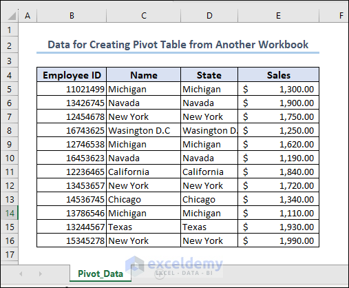
- Check out our dataset for representation.
- Insert a new module in the VBA window.
- Enter the following code into the module and Run it.
Code:
Sub CreatePivotTableFromAnotherWorkbook()
    Dim sourceWorkbook As Workbook
    Dim destinationWorkbook As Workbook
    Dim sourceWorksheet As Worksheet
    Dim destinationWorksheet As Worksheet
    Dim pivotCache As pivotCache
    Dim pivotTable As pivotTable
    ' Set the source workbook (where the data is stored)
    Set sourceWorkbook = Workbooks.Open("C:\ExcelDemy\Another Wokbook for Pivot Data.xlsx")
    ' Set the destination workbook (where the pivot table will be created)
    Set destinationWorkbook = ThisWorkbook
    ' Set the source worksheet and data range
    Set sourceWorksheet = sourceWorkbook.Worksheets("Pivot_Data")
    Set dataRange = sourceWorksheet.Range("B4:E16")
    ' Set the destination worksheet
    Set destinationWorksheet = destinationWorkbook.Worksheets("Pivot_from_Another_Workbook")
    destinationWorksheet.Activate
    ' Create a pivot cache based on the data range
    Set pivotCache = destinationWorkbook.PivotCaches.Create(SourceType:=xlDatabase, SourceData:=dataRange)
    ' Create a pivot table using the pivot cache
    Set pivotTable = pivotCache.CreatePivotTable(TableDestination:=destinationWorksheet.Range("B4"), TableName:="MyPivotTable")
    ' Set the row and column fields, as well as the values for the pivot table
    With pivotTable
        .AddDataField .PivotFields("Sales"), "Total Sales", xlSum
        .PivotFields("State").Orientation = xlRowField
        .PivotFields("Employee ID").Orientation = xlColumnField
    End With
    ' Save and close the workbooks
    sourceWorkbook.Close savechanges:=False
    destinationWorkbook.Close savechanges:=True
End Sub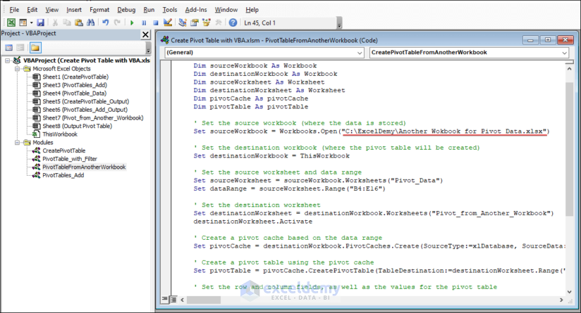
Code Breakdown:
- The code declares variables for sourceWorkbook, destinationWorkbook, sourceWorksheet, destinationWorksheet, pivotCache, and pivotTable.
- We set the source workbook by opening the workbook located at “C:\ExcelDemy\Another Wokbook for Pivot Data.xlsx“.
- Then, we set the destination workbook to the current workbook (the workbook where the code is running).
- We set the sourceWorksheet to the “Pivot_Data” worksheet in the sourceWorkbook, and the dataRange variable to the range “B4:E16” in the sourceWorksheet.
- Next, we set the destination worksheet to the “Pivot_from_Another_Workbook” worksheet in the destinationWorkbook.
- We activated the destination worksheet to ensure the pivot table is created in the correct worksheet.
- After that, we created the pivotCache based on the data range (dataRange) from the sourceWorkbook.
- We created the pivot table using the pivotCache. Then, we set the table destination to cell B4 in the destinationWorksheet, and named the table “MyPivotTable“.
- The row and column fields of the pivot table are configured. We added the “Sales” field as a data field with the “Total Sales” label. We set the “State” field as a row field and the “Employee ID” field as a column field.
- Then, we closed sourceWorkbook without saving changes and destinationWorkbook with saving changes.
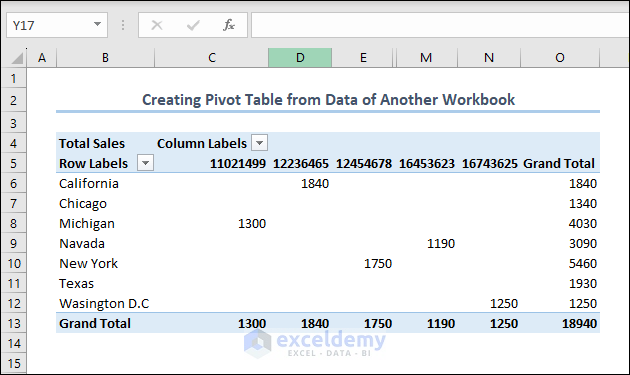
- Finally, you will see that the code has created a pivot table in the current workbook and collected data from another workbook as we instructed.
Read More: How Do I Create a Pivot Table from Multiple Worksheets
Things to Remember
- Don’t forget to save the file as an xlsm file before running the VBA code.
- In many parts of the code, we used cell references and worksheet names, and you have to adjust according to your one.
- In the last code, we accessed a closed workbook. You have to change the file directory according to your one.
Download the Practice Workbook
You can download the practice workbook from here.
Related Articles
- VBA Code to Create Pivot Table with Dynamic Range in Excel
- How to Use VBA to Create Pivot Table from Named Range in Excel
<< Go Back to How to Create Pivot Table in Excel | Pivot Table in Excel | Learn Excel
Get FREE Advanced Excel Exercises with Solutions!
