How to Create Pivot Table in Excel for Different Worksheets

Here’s an overview of a pivot table created from different worksheets.

An Example of Creating a Pivot Table in Excel

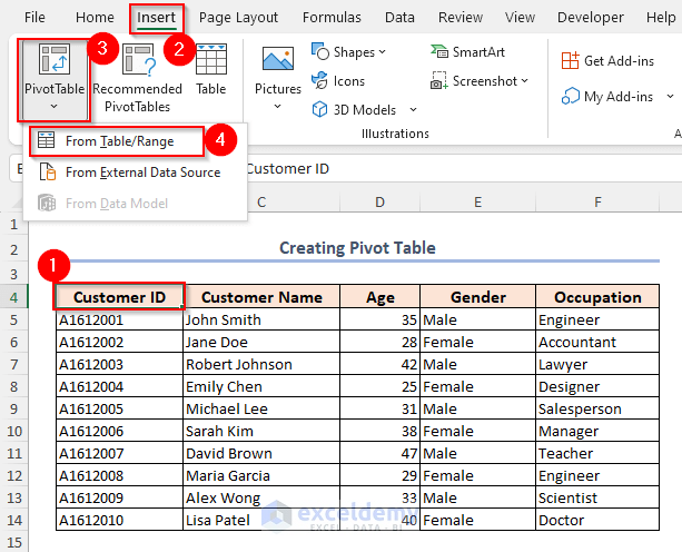
Step 1 – Insert a Pivot Table in Excel

Select the data range.
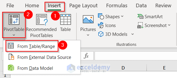
Go to the Insert tab.
Select PivotTable .
Click From Table/Range.

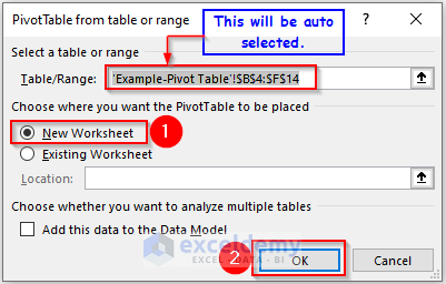
A dialog box named PivotTable from table or range will appear.

Select New Worksheet if it is not selected already.
Press OK.

A Pivot Table will be inserted into a new worksheet.

Step 2 – Add the Fields to the Pivot Table

After inserting the Pivot Table, the PivotTable Fields will appear on the right side of the screen. The PivotTable Fields task pane has two parts: the upper part, where the field names reside, and the lower part, where you will place the field names from the upper part.

Select and drag the field names (at the top of the PivotTable Fields task pane) to one of the four boxes at the bottom of the task pane.
We dragged the Customer ID into the Values area. The Pivot Table will display the total of all the values in the Count of Customer ID column.
Select and drag the field names you want in your Row Labels into the Rows area. We put the Gender, and Occupation type fields in the Rows area.

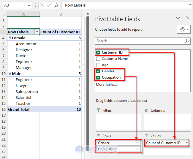
The first portion of the above figure gives the desired Pivot Table. From this Pivot Table, you can easily find out the grand total of the listed customers.

Tip: Typically, the PivotTable Fields task pane is docked on the right side of your Excel window. You can drag its title bar to move it anywhere in your Excel window. If you click a cell outside the Pivot Table, the task pane will temporarily hide.

How to Create a Pivot Table in Excel for Different Worksheets: 3 Easy Ways

Method 1 – Using the PivotTable and PivotChart Wizard to Create a Pivot Table for Different Worksheets

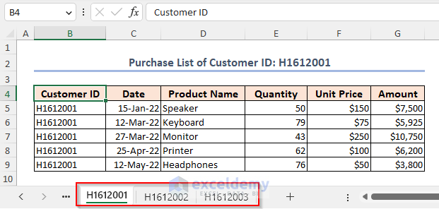
We have the purchase list of customer ID H1612001 placed in the worksheet named H1612001. We have two other similar worksheets.

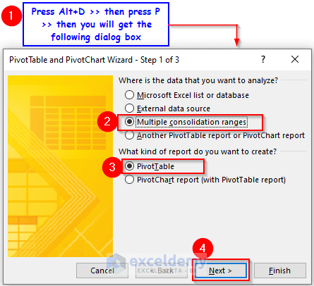
Press Alt + D, then press P.

A dialog box named PivotTable and PivotChart Wizard – Step 1 of 3 will show up.

Select Multiple consolidation ranges in the Where is the data you want to analyze? options.
Click on PivotTable in the What Kind of report do you want to create? options.
Click Next.

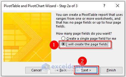
Another dialog box will open named PivotTable and PivotChart Wizard – Step 2a of 3.

Select I will create the page fields.
Click Next.

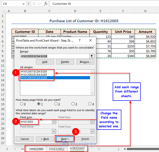
Another new dialog box will open.

From the sheet named H1612001, we selected the range of cells C4:G9.
Click on the Add options.
Put 1 in the How many page fields do you want?
Give a name for the selected range in the Field one: box. We named it H1612001.

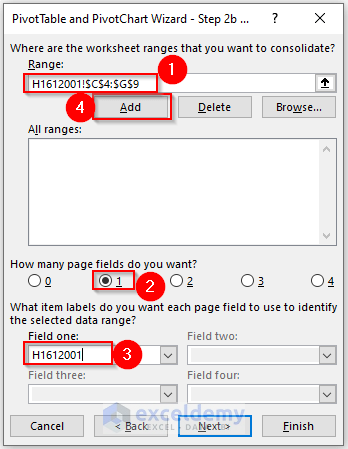
Repeat to select and add the other sheets from which you wish to create a Pivot Table. Name every single one of them.
Before naming the selected range, make sure to select the added range.
Click Next.

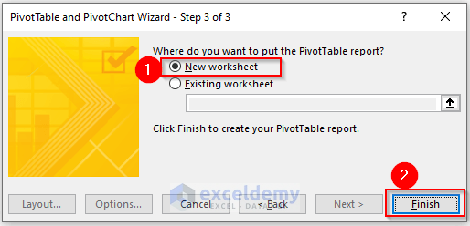
You’ll get a final window.

Select New worksheet and click on Finish.

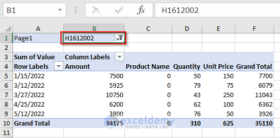
You will get a new Pivot Table containing all the data of sheets. We have the Count of Value in the Values area. We need to have the Sum instead of it.

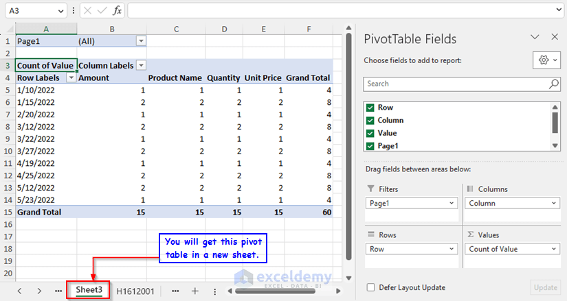
Switch the Field value from Count to Sum.

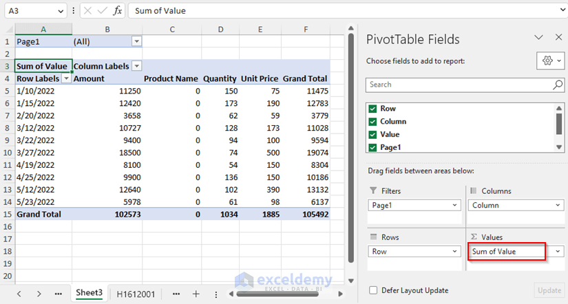
There is a Custom Filter button on top of the table. Select H1612002 from that filter.

Note: If you have alphabetical data and you choose Sum of Value in the Values area then you will get 0 in that column. One more thing, you can use different ranges of datasets.

Method 2 – Setting Relationships Between Two Excel Tables for Creating a Pivot Table Using Different Worksheets

We have Customer ID as the common column among the two datasets.

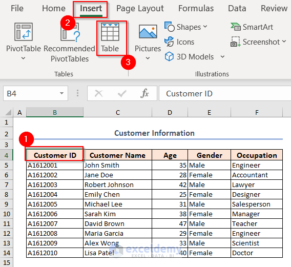
Select any cell of the dataset.
From the Insert tab, click on Table from the Tables group.

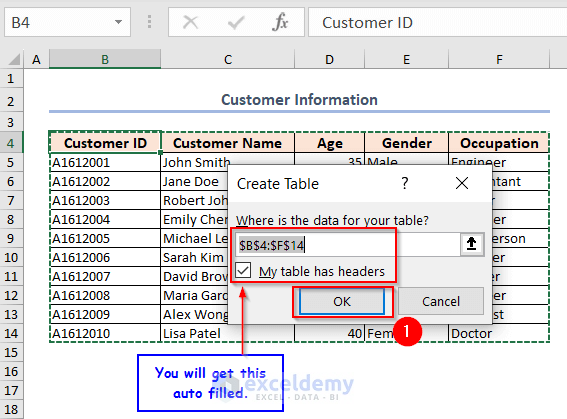
A dialog box named Create Table will appear.

You will have the range selected and My table has headers box checked.
Click OK.

You will get a table.

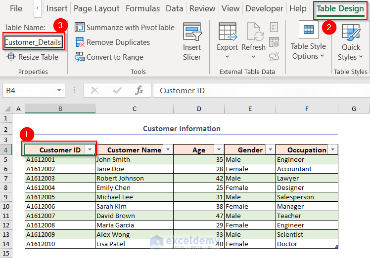
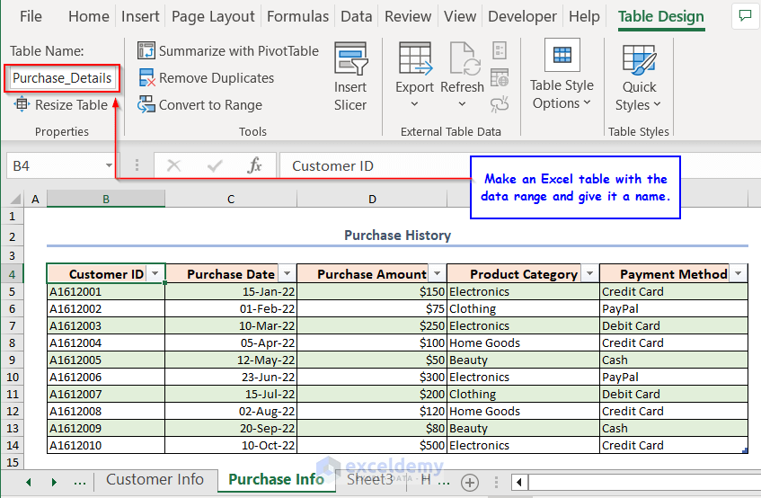
Go to the Table Design tab. To get the Table Design tab, click on any cell from the table.
Write a name in the Table Name: box.

Make another Excel table with the second dataset and give it a name.

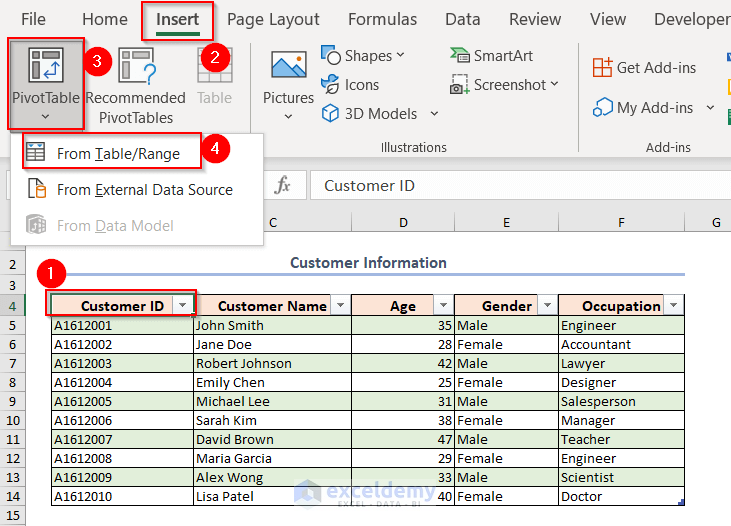
Select any cell of the Customer_Details table.
Go to the Insert tab.
Click on PivotTable.
Select From Table/Range.

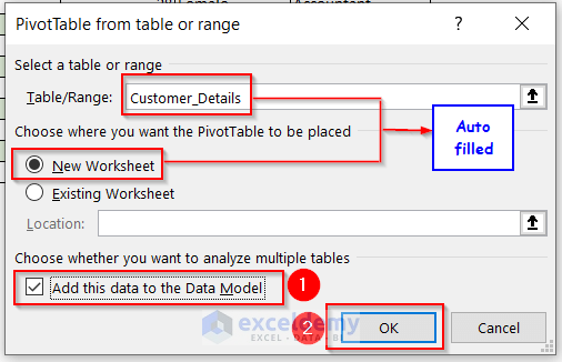
In the dialog box named PivotTable from table or range, you will get the Table/Range: box auto-filled.
Click on New Worksheet in Choose where you want the PivotTable to be placed.
Check Add this data to the Data Model.
Press OK.

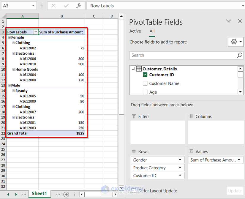
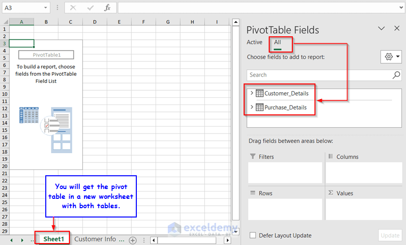
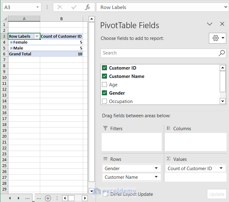
You’ll get a Pivot Table in a new worksheet with all the fields from both of the tables presented.

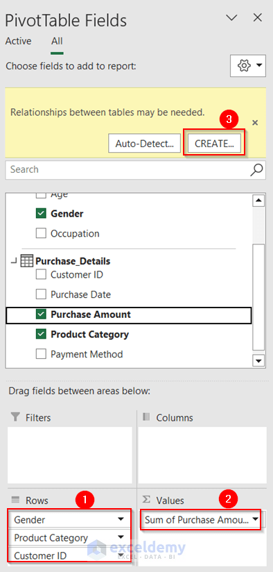
Drag the Customer ID and Gender from the Customer_Details table in the Rows field.
Drag the Product Category column from the Purchase_Details table to the Rows field and the Purchase Amount column to the Values field.
A small yellow highlight window will appear on the fields. Click on Create in that.

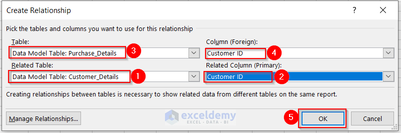
A new dialog box opens named Create Relationship.

Select the Purchase_Details as the first Table and Customer_Details as the Related Table.
In both cases, select Customer ID as the column.
Click OK.

The Pivot Table shows new values.

Method 3 – Applying Power Query to Make a Pivot Table for Different Worksheets

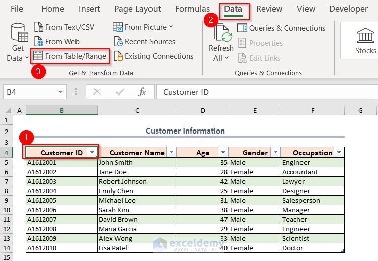
Convert the data ranges into Excel tables and give them specific names as in Method 2.
Select any cell of the Customer_Details table.
Go to the Data tab and, from the Get & Transform Data group, click on From Table/Range.

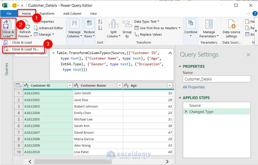
This will take the Customer_Details table into the Power Query.

Select the Home tab on the ribbon.
Select the Close & Load drop-down and choose the Close & Load To option.

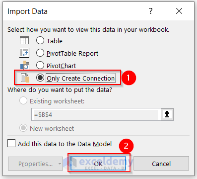
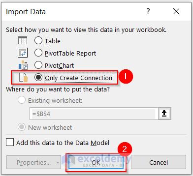
The Import Data dialog box will appear.

Select Only Create Connection from the Select how you want to view this data in your workbook section.
Click on OK.

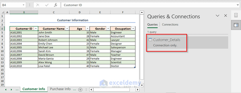
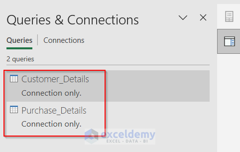
Thias will create a connection with the name of the table and appear in the Queries & Connections.

Select any cell on the second table (Purchase_Details).
Go to the Data tab and select the From Table/Range option.

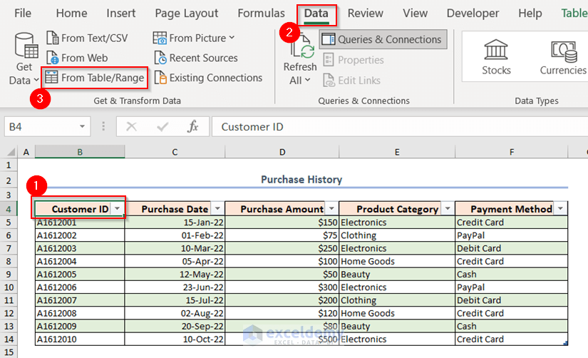
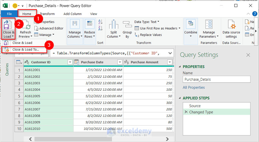
This will take the Purchase_Details table into the Power Query.

Select the Home tab and select the Close & Load To option.

You get the Import Data dialog box.

Select Only Create Connection from the Select how you want to view this data in your workbook section.
Press OK.

There are connections created between the two tables.

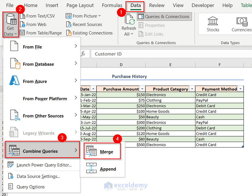
Go to the Data tab.
From the Get Data drop-down option, go to Combine Queries and select Merge.

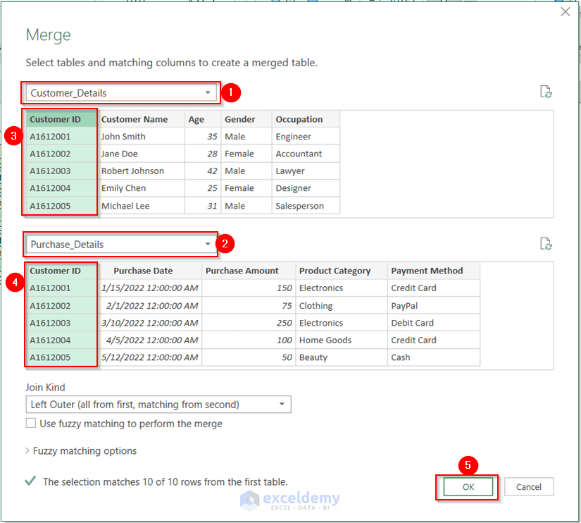
The Merge dialog box will appear.

From the first drop-down option, select the Customer_Details table.
From the second drop-down option, choose the Purchase_Details table.
Select the Customer ID column for both tables to create a connection.
Press OK.

You’ll go back to power query again.

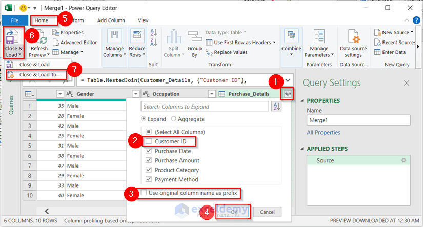
Select the two-sided arrow in the header named Purchase_Details and uncheck Customer ID and Use original column name as prefix.
Click OK.
Go to the Home tab and select the Close & Load To option.

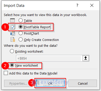
The Import Data dialog box will appear.

Select PivotTable Report from the Select how you want to view this data in your workbook section.
Select the New Worksheet option to put the data and click on OK.

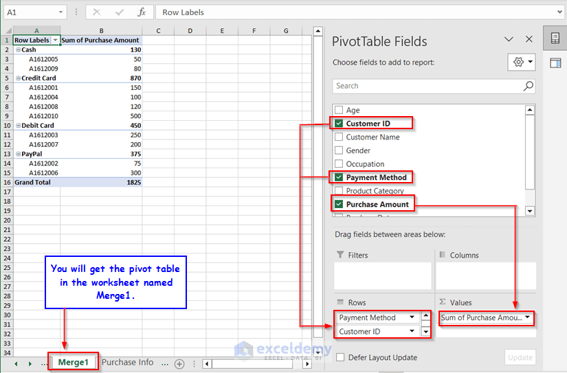
We will get a Pivot Table in a new worksheet. You must drag the fields into the areas to get the result.

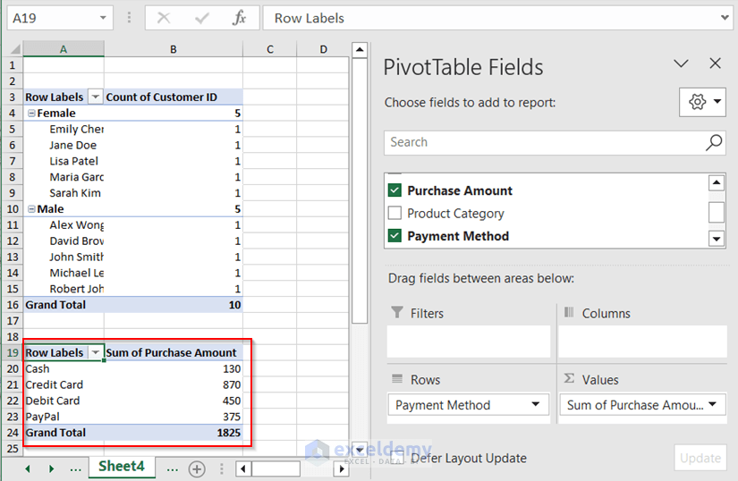
How to Create Multiple Pivot Tables on One Sheet in Excel

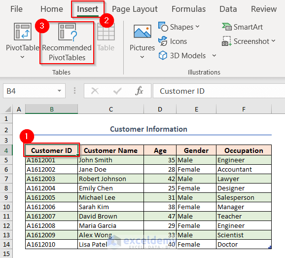
Click on any cell of the data table.
From the Insert tab, select Recommended PivotTables.

The dialog box named Recommended PivotTables will pop up.

Choose your preferred Pivot Table and press OK.

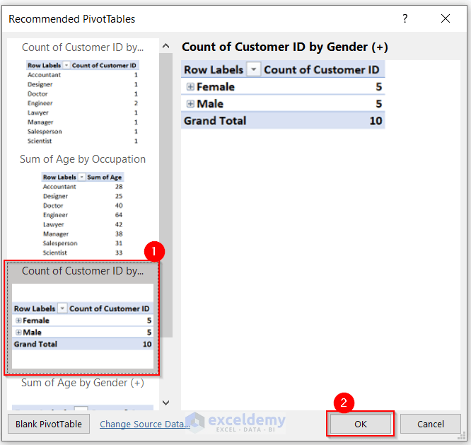
Click on the plus (+) sign to see the details of Row Labels.

Go to the Insert tab.
From PivotTable, select From Table/Range.

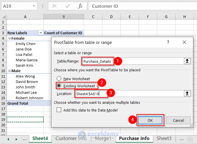
The PivotTable from table or range appears.

Write another table name in the Table/Range box, choose Existing Worksheet, set the Location, and press OK.

You must set the location while keeping enough space for the first Pivot Table.

We will get another Pivot Table in that worksheet. You must drag the fields into the areas to get the output of the 2nd Pivot Table.

Frequently Asked Question

What is the benefit of using a Pivot Table in Excel?

With a Pivot Table, you can find a summation, average value, count of data, and so on mathematical operations at a glance. Basically, you can analyze the data properly and easily with the Pivot Table. Also, you can filter the data and get value according to that. Whenever you have a large dataset, you should use the Pivot Table. Then, you can handle your data within a very short period.

Can I update the data source for a Pivot Table in Excel?

After updating the data source, click on any cell in the Pivot Table, go to PivotTable Analyze, and press Refresh.

Things to Remember

Convert the dataset into Excel tables before making a Pivot Table.
You have to manually drag the fields into areas in the PivotTable Fields task to get the Pivot Table.
If you don’t see the PivotTable Fields task panel, click on the Pivot Table, go to PivotTable Analyze, and press Field List.
In the Rows area, maintain a sequence. The first inserted column in the Rows area will get the first priority. After that, all other inserted columns will be subgrouped under that column.