Creating a Pivot Table Automatically in Excel (2 Methods)

Pivot tables allow you to easily extract insights from complex datasets, but creating them manually can be time-consuming and tedious. Fortunately, Excel provides several tools to help automate the process of creating pivot tables. In this article, we will explore two techniques: the Recommended PivotTables feature and VBA macros.

Here’s an overview of what we are going to achieve:

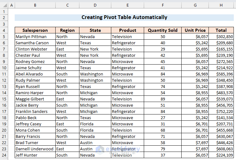
To create a Pivot Table automatically, we’ll use the following dataset which contains a company’s regional sales data.

Method 1 – Using Recommended PivotTables Feature

Microsoft introduced an exclusive feature in Excel 2013 called Recommended PivotTables. Using it, we can create many types of Pivot Tables quickly.

Steps:

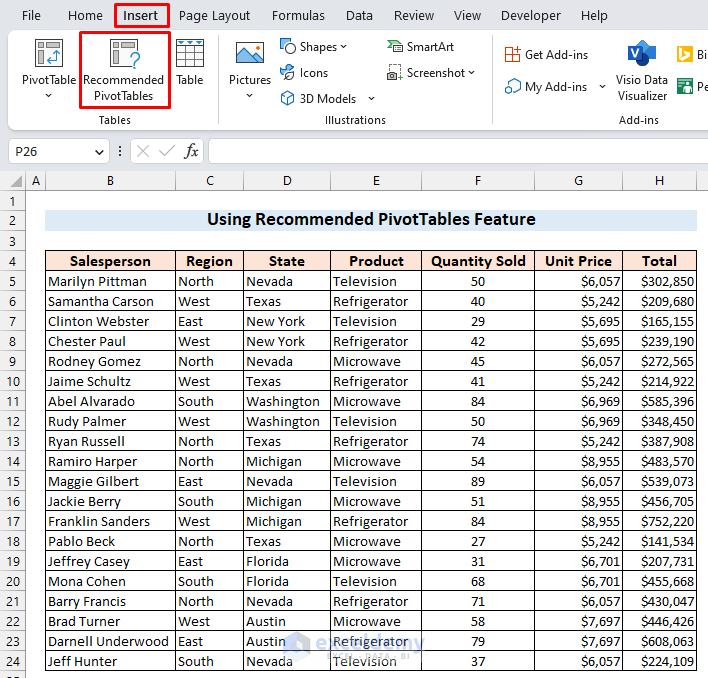
• Click on the Recommended PivotTables option from the Insert ribbon.

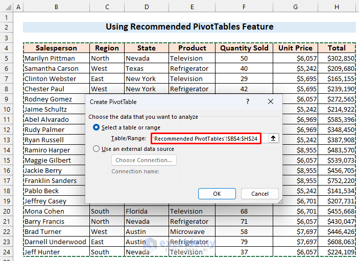
• Select the data range from your worksheet and press OK.
• Or, select any cell within the data range, choose Insert ➪ Tables ➪ Recommended PivotTables. Excel will quickly scan your data, and the Recommended PivotTables dialog box will appear.
• If you have data from an external data source then you can import it by using the Use an external data source option.

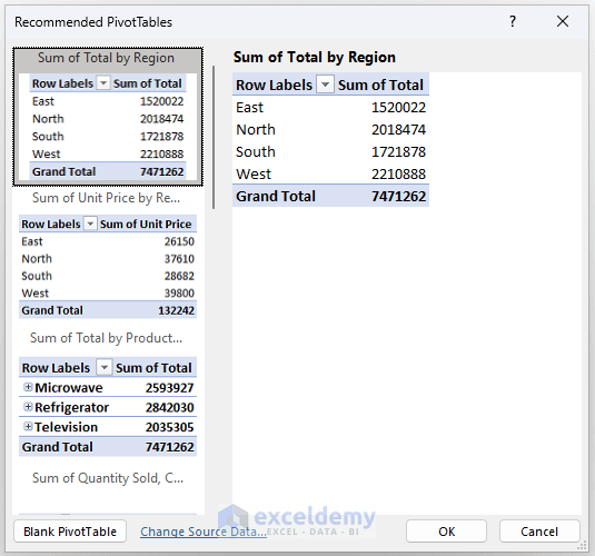
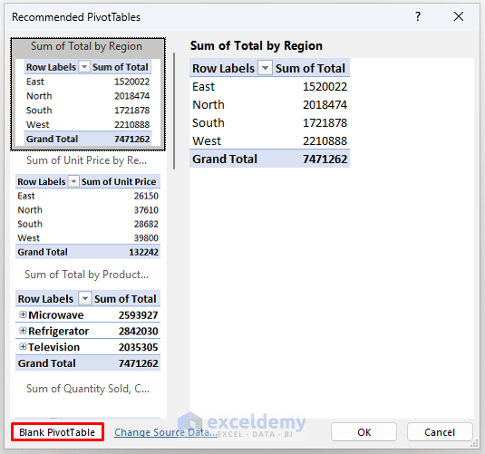
A dialog box will appear presenting thumbnails of some pivot tables.

• Select one of these options.
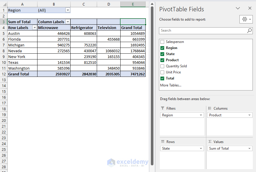
• If none of the options suit you, click on the Blank PivotTable option to open the Pivot Table fields and select the customized fields according to your requirements manually.

After clicking on the Blank PivotTable option, the main Pivot Table fields are shown like in the image below.

A customized Pivot Table is created.

Method 2 – Using a VBA Macro

When you need to insert Pivot Tables frequently, using VBA is the best option. We can set the fields in a Macro, and whenever we run the Macro, it will create a new Pivot Table with a single click while deleting the previous one.

Steps:

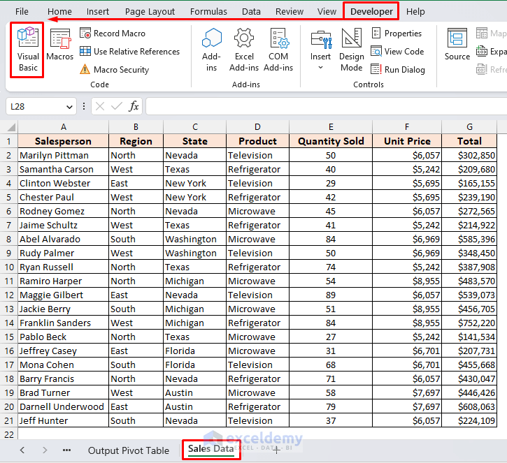
• Place the dataset so that its starts at cell A1.

We changed the sheet name to ‘Sales Data’, and we’ll use this sheet name in our codes. So, if you have another name then don’t forget to update it.

• Click on the Visual Basic command from the Developer ribbon.

• Open a new module by clicking Insert > Module.

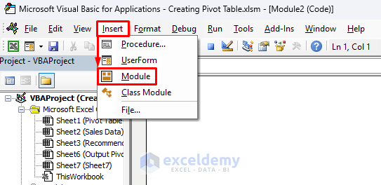
• Enter the following code in the module:

Sub Create_PivotTable_Automatically()
Dim PV_Sheet As Worksheet, DS_Sheet As Worksheet
Dim PV_Cache As PivotCache
Dim PV_Table As PivotTable
Dim PV_Range As Range
Dim LtRow As Long, LtColumn As Long
Dim xSheet1 As Variant
On Error Resume Next
With Application
    .DisplayAlerts = False
    .ScreenUpdating = False
End With
For Each xSheet1 In ActiveWorkbook.Worksheets
    If xSheet1.Name = "Output Pivot Table" Then
        xSheet1.Delete
    End If
Next xSheet1
Worksheets.Add.Name = "Output Pivot Table"
Set PV_Sheet = Worksheets("Output Pivot Table")
Set DS_Sheet = Worksheets("Sales Data")
LtRow = DS_Sheet.Cells(Rows.Count, 1).End(xlUp).Row
LtColumn = DS_Sheet.Cells(1, Columns.Count).End(xlToLeft).Column
Set PV_Range = DS_Sheet.Cells(1, 1).Resize(LtRow, LtColumn)
Set PV_Cache = ActiveWorkbook.PivotCaches.Create(SourceType:=xlDatabase, SourceData:=PV_Range).CreatePivotTable(TableDestination:=PV_Sheet.Cells(2, 2), TableName:="Automatically Created PivotTable")
Set PV_Table = PV_Cache.CreatePivotTable(TableDestination:=PV_Sheet.Cells(1, 1), TableName:="Automatically Created PivotTable")
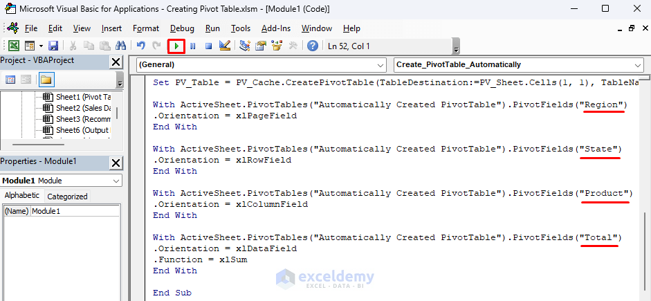
With ActiveSheet.PivotTables("Automatically Created PivotTable").PivotFields("Region")
.Orientation = xlPageField
End With
With ActiveSheet.PivotTables("Automatically Created PivotTable").PivotFields("State")
.Orientation = xlRowField
End With
With ActiveSheet.PivotTables("Automatically Created PivotTable").PivotFields("Product")
.Orientation = xlColumnField
End With
With ActiveSheet.PivotTables("Automatically Created PivotTable").PivotFields("Total")
.Orientation = xlDataField
.Function = xlSum
End With
End Sub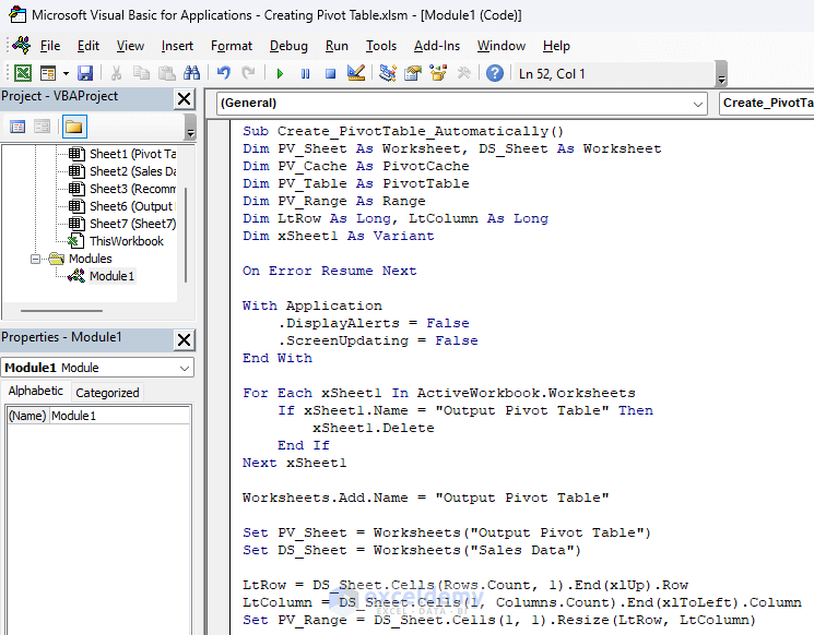

• In the last section of our code, we declare the ‘Region’ heading to filter sales data by the regions, ‘State’ for the row field, ‘Product’ for the column field, and ‘Total’ for the value field.
• If you have different headings, change these values to match your required fields.
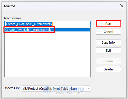
• Run the code by clicking on the Play icon or pressing F5.

• Select the macro name and click on the Run button.

A Pivot Table in a new sheet named ‘Output Pivot Table’ is created.

• Change this sheet name in the code if desired.

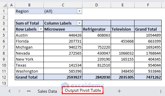
• From the upper drop-down option, change the filter by region.

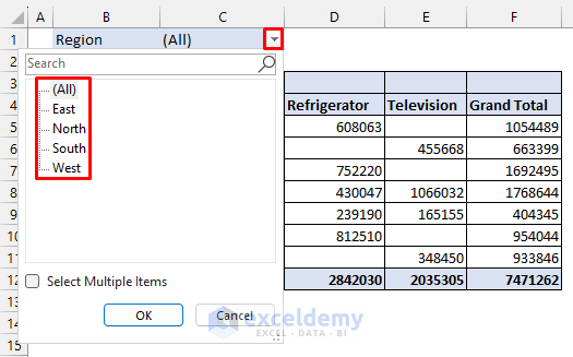
Here’s the filtered Pivot Table for the ‘South’ region.

Read More: How to Use Excel VBA to Create Pivot Table

Frequently Asked Questions

1. Can you use a macro to create a Pivot Table?

Yes, refer to Method 2 above.

2. How to auto-refresh Pivot Table every 5 minutes?

Refer to the following article:

How to Auto Refresh Pivot Table without VBA in Excel

3. Can you make a pivot of a Pivot Table?

Yes, this technique is called “nested pivoting” or “double pivoting”. Follow these steps:

• Create a pivot table with the desired data fields and column/row labels.
• Add additional fields to the pivot table by dragging them to the “Values” section of the PivotTable Fields pane.
• Right-click on any cell in the pivot table and select “Show Details” from the context menu.

Excel will create a new worksheet with a table of detailed data for the selected cell(s).

• Create a new pivot table based on this detailed data table by selecting the data and choosing “Insert PivotTable” from the “Tables” group in the “Insert” tab.
• Customize the new pivot table by selecting the desired fields and column/row labels and applying any necessary calculations or formatting.

Download Practice Workbook

Related Articles

• How to Insert A Pivot Table in Excel
• How to Create Pivot Table Report in Excel
• How to Create Pivot Table in Excel for Different Worksheets
• How Do I Create a Pivot Table from Multiple Worksheets
• VBA Code to Create Pivot Table with Dynamic Range in Excel
• How to Use VBA to Create Pivot Table from Named Range in Excel

<< Go Back to How to Create Pivot Table in Excel | Pivot Table in Excel | Learn Excel