How Do I Create a Pivot Table from Multiple Worksheets – 2 Methods

The dataset contains sales statistics.

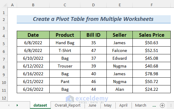
To convert it to a table:

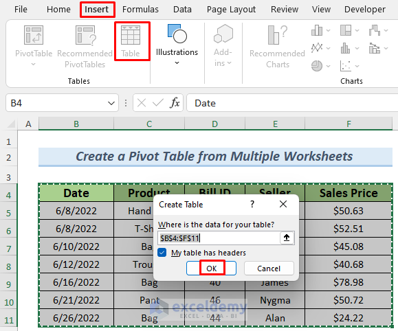
• Select the dataset and go to Insert >> Table.
• Check My table has headers and click OK. (You can also press CTRL+T to convert the dataset to a table).

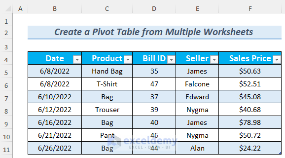
This is the output.

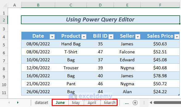
Method 1 – Using the Power Query Editor to Create a Pivot Table from Multiple Worksheets

Steps:

• Use the following sheets to insert a Pivot Table.

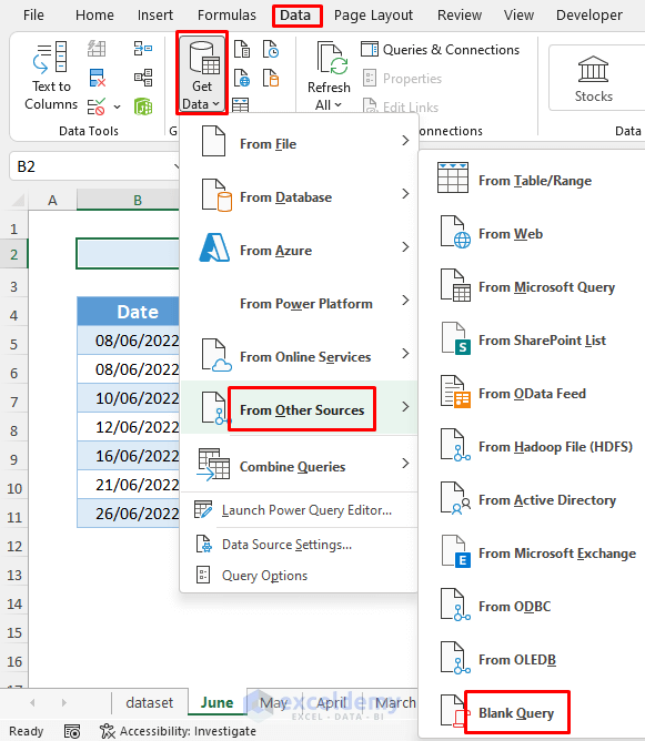
• Go to Data >> Get Data >> From Other Sources >> Blank Query.

• In the Power Query Editor, name your Query. Here, I named Overall_Report.
• Press ENTER.
• Enter the following formula in the Power Query formula bar and press ENTER.

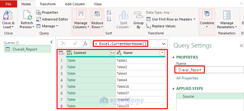
The formula will return all the tables in the workbook.

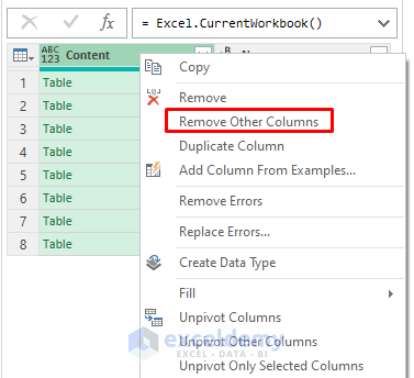
• Right-click the header of the first column.
• Remove the second column using Remove Other Columns.

• Go to Home >> Keep Rows >> Keep Top Rows.

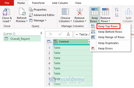
• In the Keep Top Rows window, select four (the first four tables).

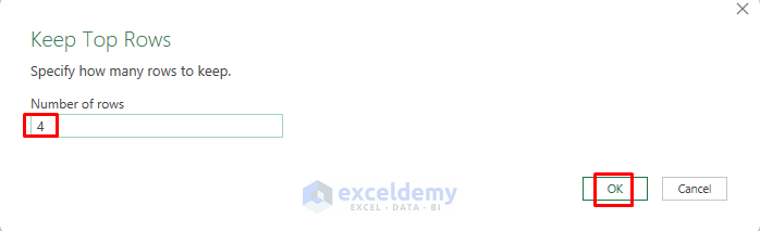
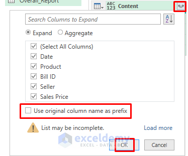
• It will return the first four rows only. Click the icon marked below.
• Uncheck Use original column name as prefix.
• Click OK.

You will see all the consolidated data in the Power Query Editor.

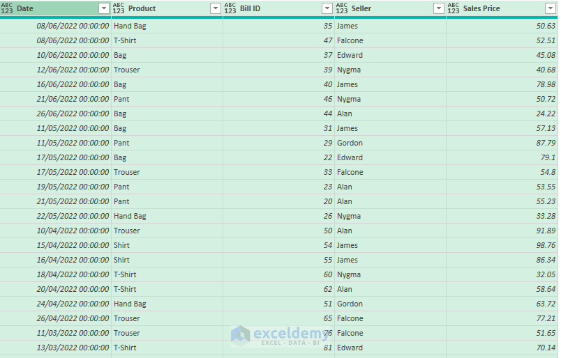
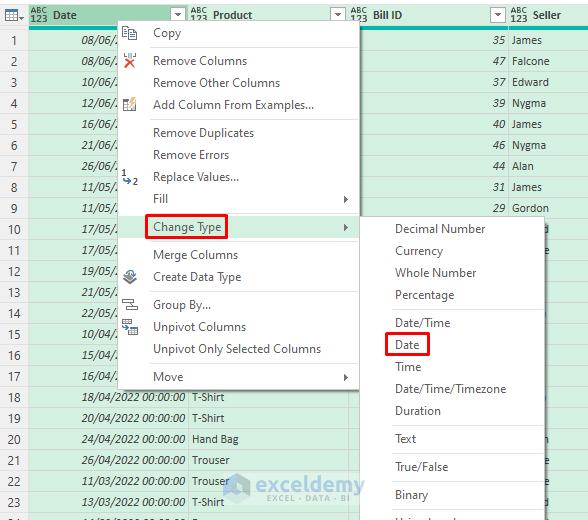
The query contains unnecessary formatting like date and time. To remove it:

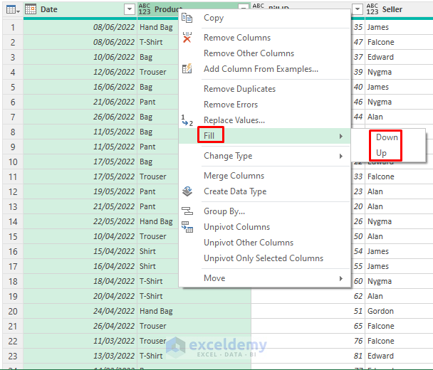
• Right-click and select the Date column.
• Choose Change Type >> Date.

• Select the columns that contain blanks and right-click >> Fill. Select Down or Up.

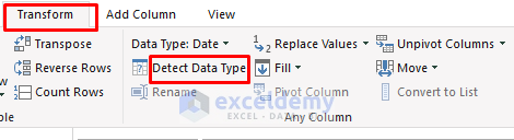
• Press CTRL+A and go to Transform >> Detect Data Type.

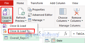
• Go to Home >> Close & Load To…

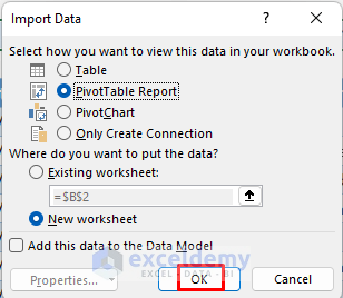
• In the Import Data dialog box, select PivotTable Report.
• Click OK.
• Select New Worksheet.

Your Pivot Table will be displayed in a new worksheet.

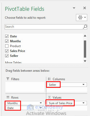
• Drag the Date range to Rows, Sales Price to Values, and Seller to Columns.

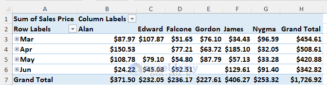
The monthly and overall sales reports from March to June are displayed. You can also see the sales records based on sellers.

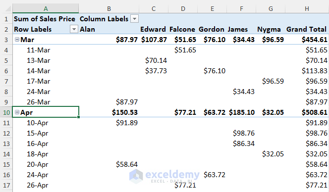
• Click the Plus button next to month to see more details about sales in that month.

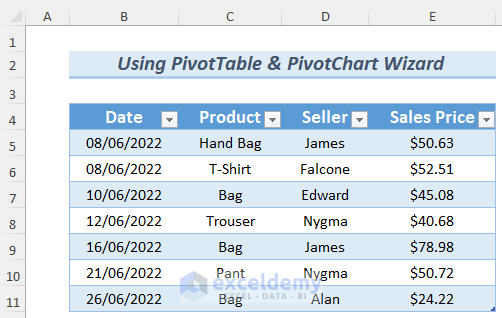
Method 2 – Using the PivotTable and PivotChart Wizard to Create a Pivot Table from Multiple Worksheets

Steps:

• Use the same worksheets but skip the Bill ID field.

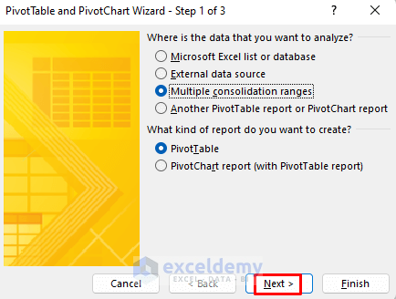
• Press ALT, D, and P, and you will see the PivotTable and PivotChart Wizard.
• Choose the area to perform data analysis. Here, Multiple consolidation ranges and PivotTable. To conduct a thorough analysis, select  PivotChart report instead of PivotTable.
• Click Next.

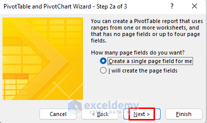
• Select Create a single page field for me.
• Click Next.

• Enter the table ranges: select the sheet that contains the sales report and choose the table. Here, the table in June (2).
• Click Add.

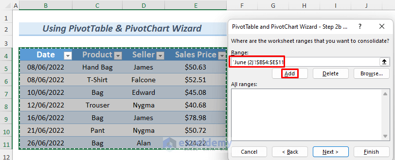
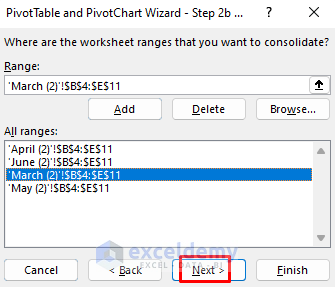
• Add the other tables.
• Click Next.

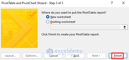
• Select New worksheet or Existing worksheet.
• Click Finish.

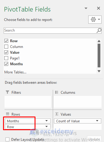
• In the PivotTable Fields, Row refers to the dates and Value refers to the sales values. So, drag the Row to Rows and Value to Values.

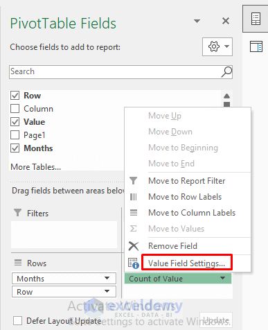
• The value field of sales values is in Count of Value. To get the sales values and their total, click Count of Value >> Value Field Settings.

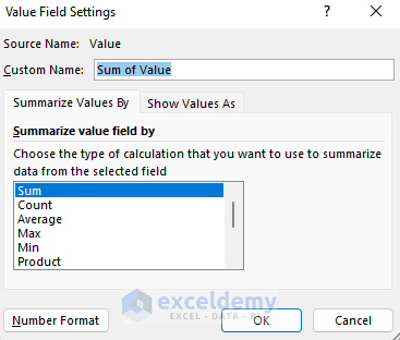
• In the Value Field Settings window, choose Sum of Value and click OK.

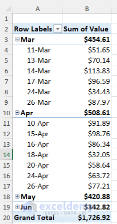
A monthly sales report is displayed in the Pivot Table.

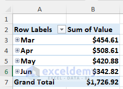
• To get a daily analysis, click the Plus icon beside month name.

Read More: How to Create Pivot Table in Excel for Different Worksheets

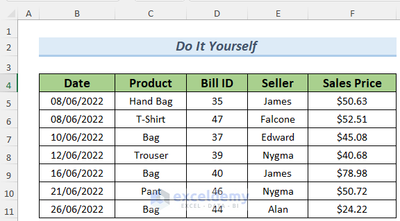
Practice Section

Practice here.

Download Practice Workbook

Related Articles

• Creating a Pivot Table Automatically in Excel
• How to Create Pivot Table Report in Excel

<< Go Back to How to Create Pivot Table in Excel | Pivot Table in Excel | Learn Excel