In Excel, we need to make a table where we must arrange a data range in a structured form. So that we don’t need to format each cell every time. In the table, all data will be in the same format as per the given instruction.
Make a Table in Excel: 2 Simple Ways
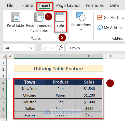
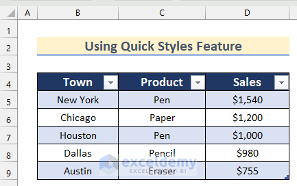
Here, we will have a data set of Products sold in different Towns with their Sales values. Data on these sheets are not very significant. We introduced that data so that you can understand it easily.
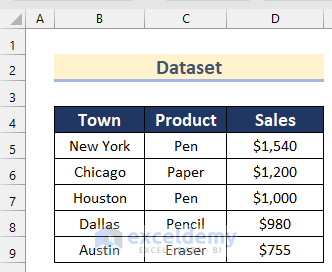
Now, we will use this organized dataset to show you how to create a table in Excel. However, make sure to have the same type of data within a column and remove blank cells before converting data range to a table.
1. Use Format as Table Feature to Make a Table in Excel
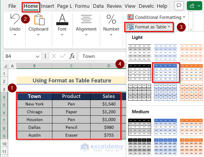
In the first method, we will use the Format as Table feature from the Home tab to make a table. Follow the steps given below to do it on your own dataset.
Steps:
- Firstly, select your desired cell range. Here, we will select cell range B4:D9.
- Secondly, go to the Home tab >> click on Format as Table >> select any table from there according to your choice.
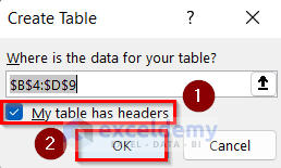
- Now, the Create Table box will open, where you will see that the data has already been selected.
- After that, turn on My table has header option.
- Lastly, click on OK.
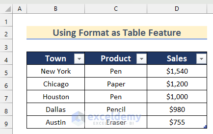
- Thus, you can make a table using your dataset.
2. Utilize Table Feature from Insert Tab to Create Table
You can also make a table utilizing the Table feature from the Insert tab in Excel.
Here are the steps.
Steps:
- In the beginning, select the cell range that you want to make a table.
- After that, go to the Insert tab >> click on Table.
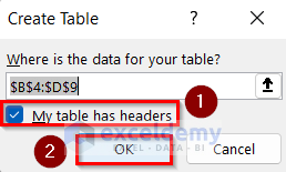
- Next, the Create Table box will appear.
- Then, turn on My table has header option.
- In the following step, click on OK.
- Finally, you will get a table using your dataset.

How to Format Table in Excel
There are many options available on the table. Let’s go through the options below and have a look at the screenshots to get a detailed idea of how to format an Excel table with some user-defined structures.
1. Use Quick Styles Feature
We have a quick style option on Table. You can use it to choose different types of table formats. Go through the steps to do that.
Steps:
- Firstly, click on the cell of the table.
- Now, we will get the Table Design option in the ribbon.
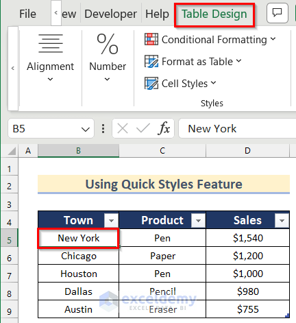
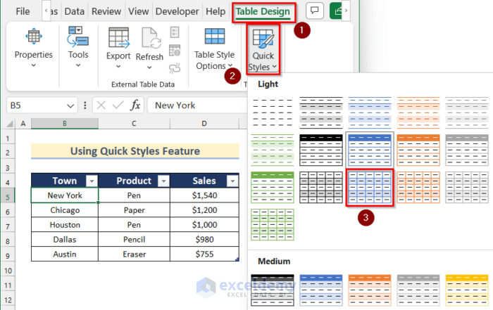
- Then, go to the Table Design tab >> click on Quick Styles.
- After clicking Quick Styles we will get a drop-down.
- From the drop-down, select a style.
- Here, we selected the Light Blue, Table Style Light 16 style.
- Finally, you can use the Quick Styles feature to style a table in Excel.
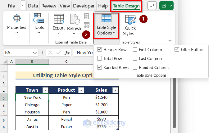
2. Utilize Table Style Options
Additionally, you can also change the table format utilizing the Table Style option.
Steps:
- Firstly, open the Table Design tab by clicking on any cell of the table.
- After that, clicking on Table Design, we will get Table Style Options.
- Thus, you can format your rows and columns in the table using the given options.
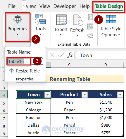
3. Rename Table from Table Design Tab
Moreover, we can rename our table from the Table Design tab. The steps are described below.
Steps:
- To start with, go to the Table Design tab >> expand the Properties option.
- Now, we will get the Table Name.
- Then, you can change the name of the table according to your wish.
4. Resize Table Using Table Design Tab
We’ll now show you how to resize your Table.
Steps:
- In the beginning, click on a cell of the table to get the Table Design option in the ribbon.
- Then, go to the Table Design tab >> expand Properties option >> click on Resize Table.
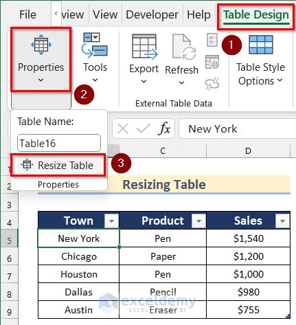
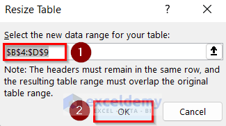
- Now, we will get the Resize Table box.
- After that, you can change the data range if you want.
- Lastly, click on OK.
5. Filter Data from Table
We can also apply Filter in Table. Here are the steps to do that.
Steps:
- Firstly, select the Filter button (down arrow sign) and you will get Filter options.
- After that, turn on or off options according to your wish.
- Here, we filtered only the data for Chicago and Dallas.
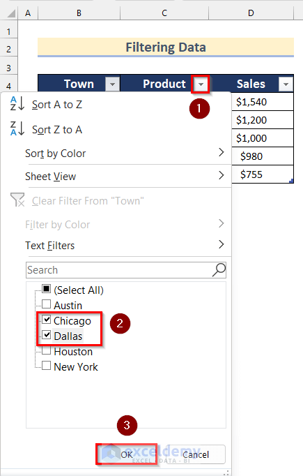
- Thus, you can filter your data from a table in Excel.
6. Use Other Additional Tools
Additionally, you can also use other tools on your table. Here are the steps to find those tools.
Steps:
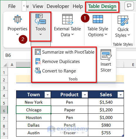
- In the beginning, go to the Table Design option >> expand Tools.
- Then, you will have the following options like:
- Summarize with PivotTable
- Remove Duplicates
- Convert to Range
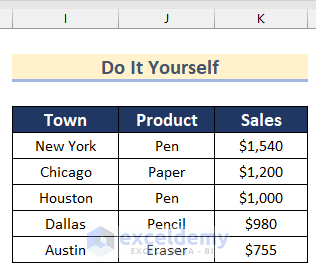
Practice Section
In this section, we are giving you the dataset to practice on your own and learn to use these methods.
Download Practice Workbook
You can download the workbook to practice yourself.
Conclusion
Here we showed how to make a Table in Excel. We also showed different options of Table in brief so that users get an idea of which things are possible to do with Table. Lastly, feel free to comment if something seems difficult to understand. Additionally, let us know any other approaches that we might have missed here. Thank you!
Make Table in Excel: Knowledge Hub
- Create Table in Excel Using Shortcut
- Create a Table in Excel Based on Cell Value
- How to Create a Table with Existing Data
- How to Create a Table Without Data
- How to Create a Table with Merged Cells
- How to Create a Table in Excel with Multiple Columns
- How to Make a Table in Excel with Lines
- How to Create a Table with Subcategories
- How to Add New Row Automatically in an Excel Table
- How to Create Table from Another Table
- How to Create Table from Another Table with Criteria
- How to Mirror Table on Another Sheet
- How to Create Table from Multiple Sheets
- How to Create a Lookup Table
- How to Make 3D Table
- How to Make a Conversion Table
- How to Make a Decision Table
- How to Create a League Table
- How to Make a Table Bigger
<< Go Back to Excel Table | Learn Excel
Get FREE Advanced Excel Exercises with Solutions!
