Create a Table in Excel Based on Cell Value (4 Easy Methods)

Method 1 – Using Table and Pivot Table to Create a Table in Excel Based on Cell Value

We will first insert a Table using our dataset, and use a Pivot Table to create a table in Excel based on cell value.

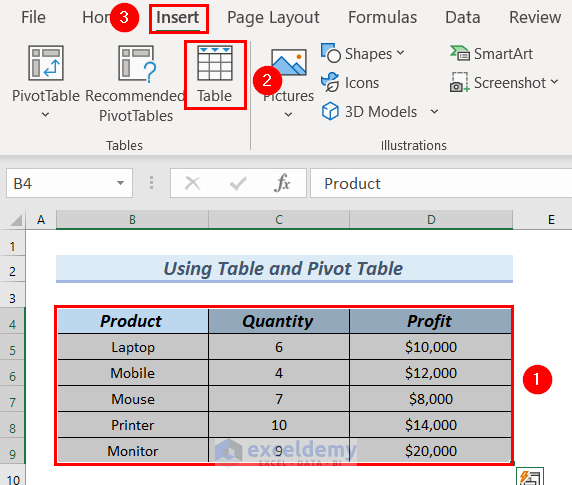
Step 1: Inserting Table

Select the dataset >> go to the Insert
From the Tables group >> select Table.

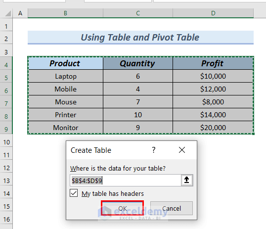
A Create Table dialog box will pop up.

Ensure that My table has headers is ticked.

Click OK.

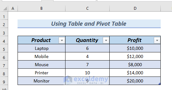
The Table will be created.

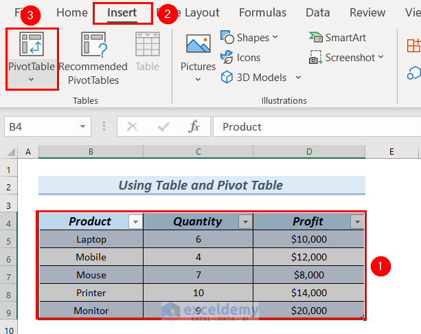
Step 2: Inserting Pivot Table

Select the data of the Table >> go to Insert.
From the Tables group >> select PivotTable.

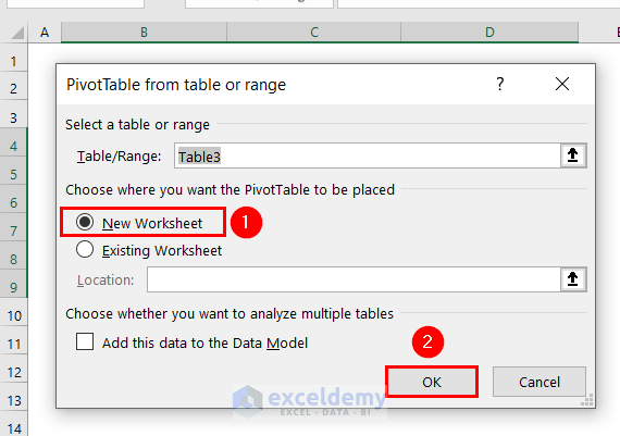
A PivotTable from table or range dialog box will be displayed.

Select New Worksheet.
Click OK.

From the PivotTable Fields >> drag Product under the Row group.
Drag Profit under the Values group.

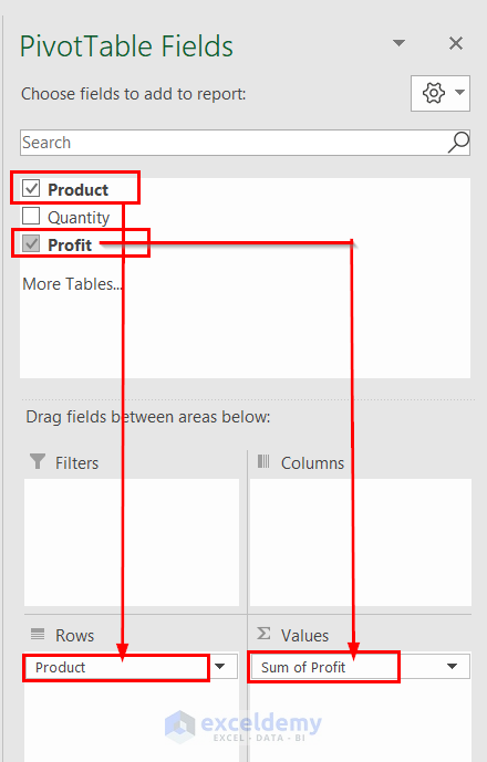
The Pivot Table will be created.

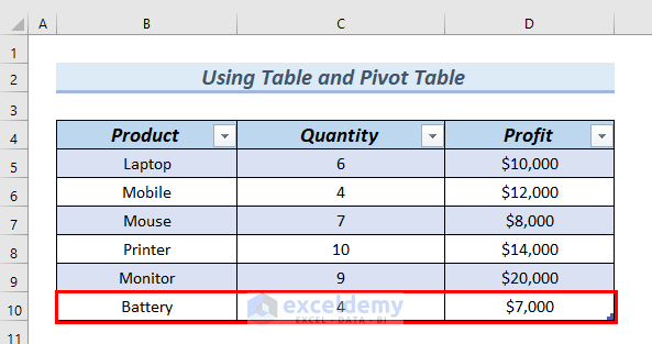
Step 3: Adding Cell to Table

We will add the product Battery in cell B10, Quantity and Profit for the product in cells C10 and D10.

Go to the Pivot Table.

Refresh the data of the Pivot Table.

Click on a cell of the Pivot Table >> go to PivotTable Analyze.
From the Data group >> select Refresh >> select Refresh.

You can also Refresh the Pivot Table data by pressing ALT+F5.

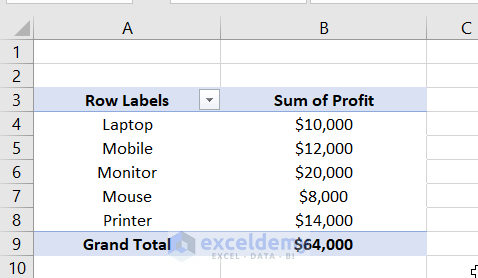
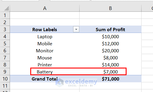
You will be able to see the product Battery along with its Profit in the Pivot Table.

You can create a table in Excel based on cell value. The result is as shown in the image below.

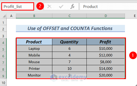
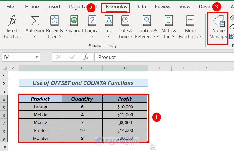
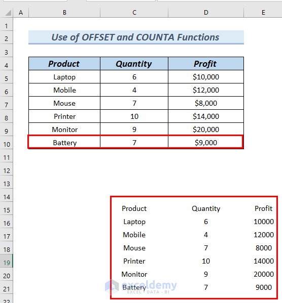
Method 2 – Use of OFFSET and COUNTA Functions to Create a Dynamic Table Based on Cell Value

Step 1: Copying Dataset to Another Location

Select the cells B4:D9 >> in the Name Box we have entered Profit_list.

To copy the data of the dataset, enter the following formula in cell C14.

=Profit_list

Press ENTER.

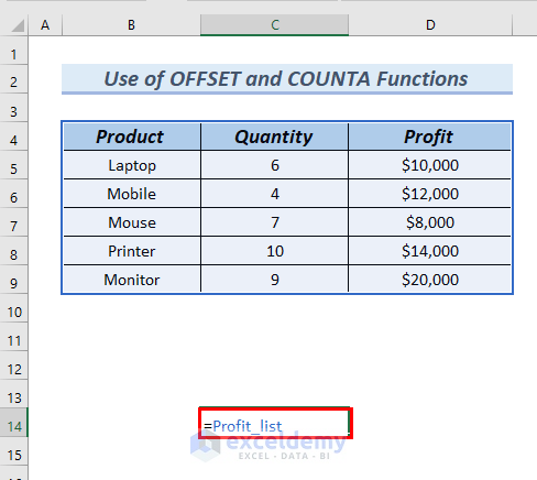
The dataset will be copied and pasted as shown below.

Step 2: Adding Cell to Dataset

.We will add the product Battery in cell B10, Quantity and Profit for the product in cells C10 and D10.

However, the copied dataset will not be updated.

Step 3: Adding Formula

In order to update the copied cells as we add a value to the dataset, we will use a formula using the OFFSET and COUNTA functions.

Select the dataset >> go to Formulas.
Select Name Manager.

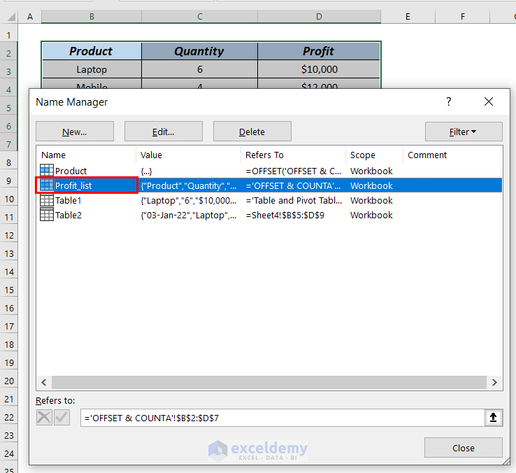
A Name Manager dialog box will pop up.

Double-click on Profit_list.

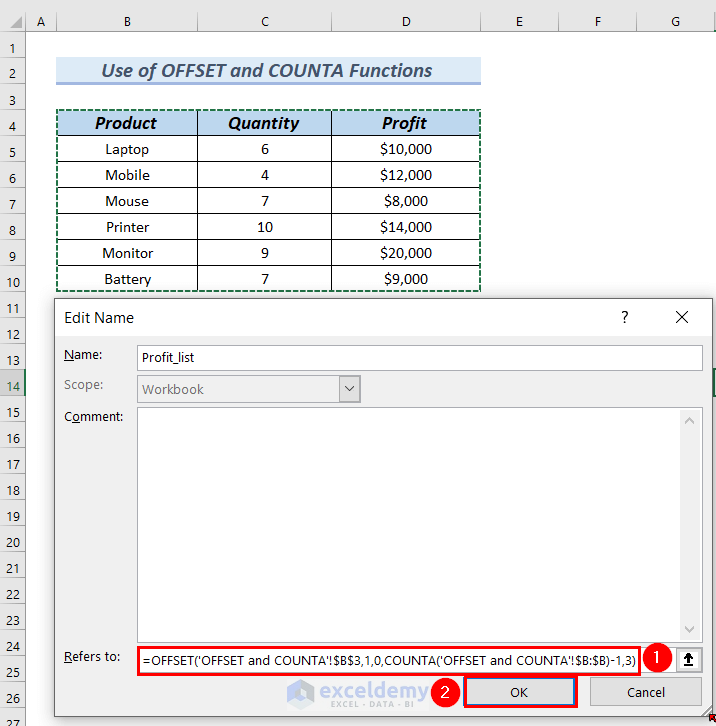
An Edit Name dialog box will pop up.

In the Refers to box, enter the following formula.

=OFFSET('OFFSET and COUNTA'!$B$3,1,0,COUNTA('OFFSET and COUNTA'!$B:$B)-1,3)

The OFFSET function returns a section from a dataset situated at a specific number of rows down and a specific number of columns right from a given cell reference.

In a specific cell range, the COUNTA function calculates the total cells which are not empty.

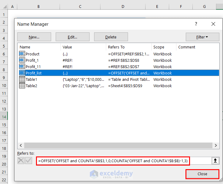
Click OK in the Edit Name dialog box.

Click Close in the Name Manager dialog box.

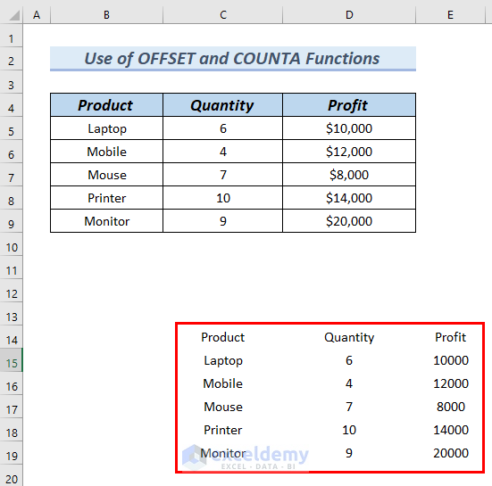
Enter Battery in cell B10, Quantity and Profit for the product in cells C10 and D10.

You will see that the copied will be updated as shown in the image below.

Method 3 – Using Filter Feature to Create a Table in Excel Based on Cell Value

Follow Step-1 of method-1 to insert a Table using the following dataset.

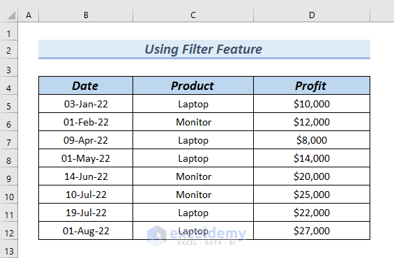
The Table will be inserted.

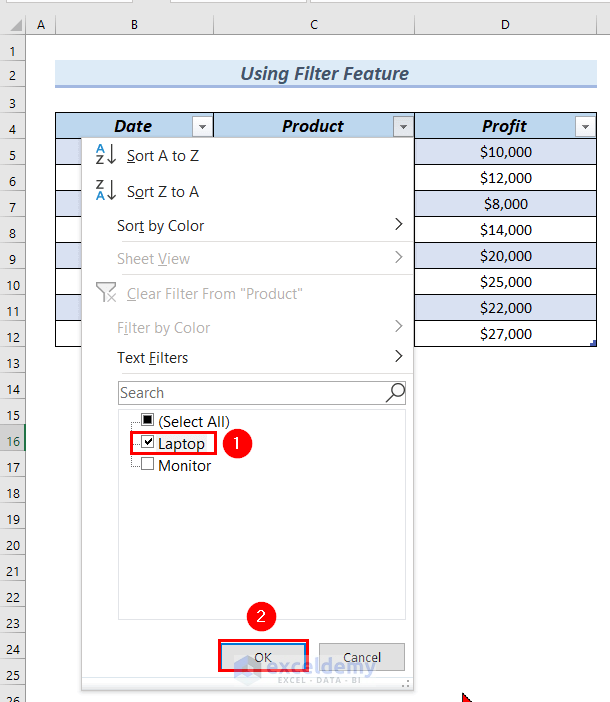
Click on the drop-down arrow of the Product column.

You can see both the products as Select All is marked.

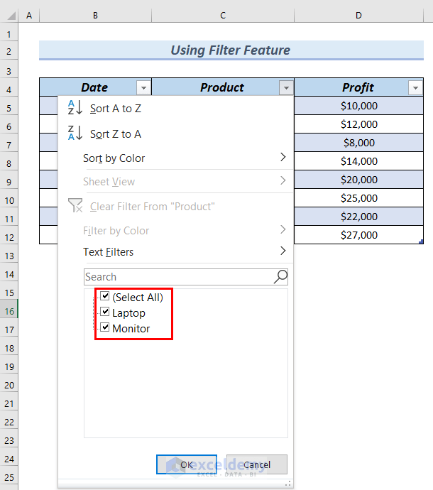
Untick the Select All option.

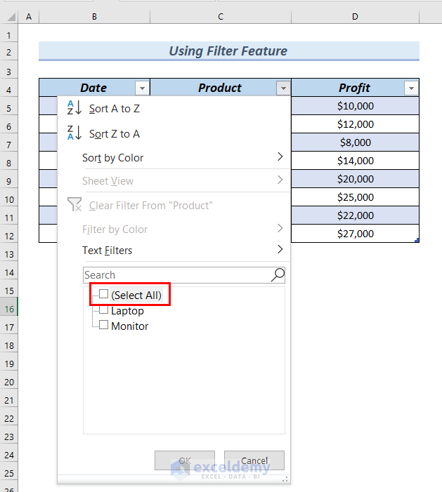
Tick on Laptop >> click OK.

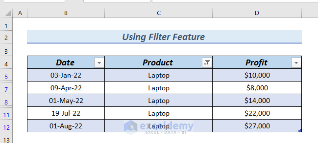
You will see that the Table will show only the dataset of laptops.

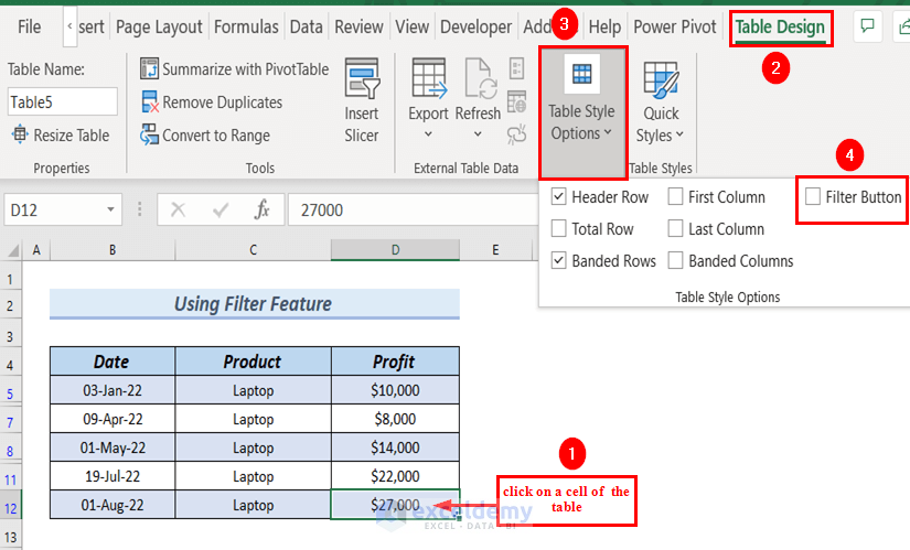
To remove the drop-down arrow from the Table.

Click on any cell of the Table >> go to Table Design.
From Table Style Options >> unmark Filter Button.

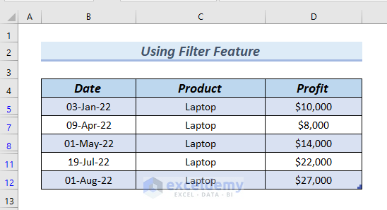
The result will be as shown in the image below.

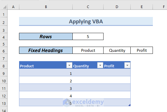
Method 4 – Applying VBA to Create a Table Based on Cell Value

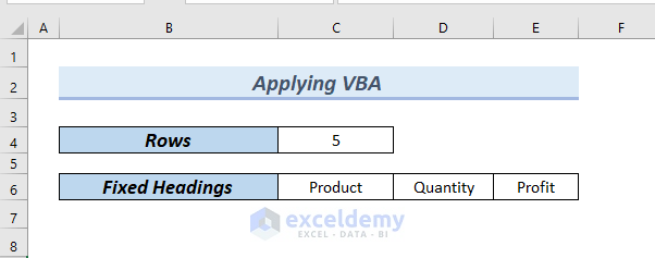
In the following image, you can see that we have to create a Table with 5 Rows and the table must have the Product, Quantity and Profit as Fixed Headings. We will use VBA code to create a table in Excel based on cell value.

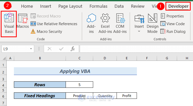
Go to the Developer tab >> select Visual Basic.

The VBA editor window will pop up (shortcut key is ALT+F11).

From the Insert tab >> select Module.

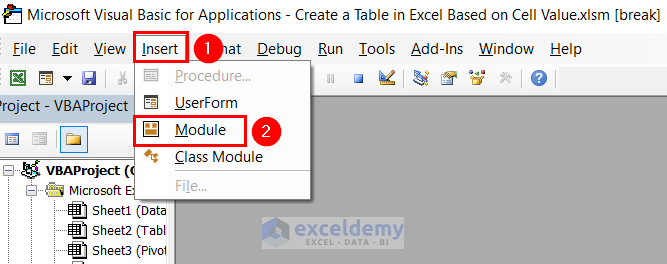
Enter the following code in the Module.

Sub Create_Table_based_on_cell()
  Dim heading() As Variant
  Dim number_of_rows As Long
  Dim number_of_column As Long
  Dim heading_color As Long
  Dim heading_row As Long
  Dim work_sheet As Worksheet
  Dim p As Long, q As Long
  Dim cell_rng As range

  Set work_sheet = ActiveSheet
  number_of_rows = work_sheet.range("C4")
  number_of_column = work_sheet.range("C5")
  heading_row = 8

  With work_sheet
  heading = .range(.Cells(6, "C"), Cells(6, "C").End(xlToRight)).Value
  heading_color = UBound(heading, 2)
  .range("B" & heading_row).Resize(1, heading_color).Value = _
  Application.Index(heading, 1, 0)
     For q = 1 To number_of_rows
        .Cells(q + heading_row, 2).Value = q
     Next q

    Set cell_rng = range("B" & heading_row).CurrentRegion

  End With

  work_sheet.ListObjects.Add(xlSrcRange, cell_rng, , xlYes).Name = "Product"

End Sub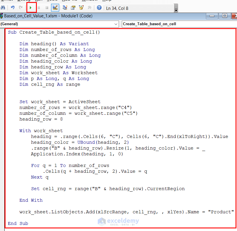

Code Breakdown

We have entered Create_Table_based_on_cell as Sub.
We have declared several variables.
We have Set the numer_of_row, numer_of_column and heading_row.
We have used a With Statement to avoid repetition of the same variable.
To select the headings by using Cell range and xlToRight properties from the sheet based on which the Table is created.
We have colored the headings and rows by using the Index
We have used the For loop to run the code until it finds the last column.
We have Named the created table as Product.

Click on the Run button to run the code.

The Table will be created based on cell value as shown in the image below.

Download Practice Workbook

Creating a Table Based on Cell Value.xlsm

<< Go Back to Excel Table | Learn Excel

Get FREE Advanced Excel Exercises with Solutions!