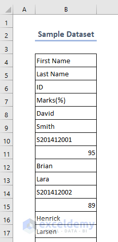
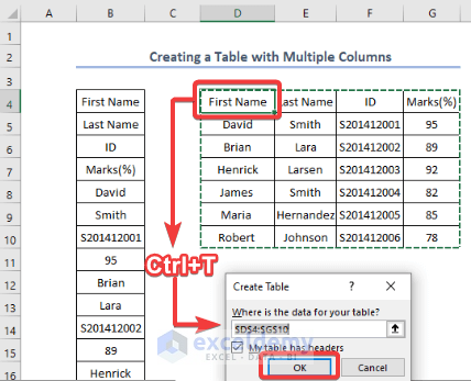
We have a column with First and Last Names, ID, and their respective marks in a single column, starting with B4. We will convert this into a table with 4 columns, each for First Name, Last name, ID, and Marks, respectively.
Method 1 – Apply a Formula with OFFSET, COLUMNS, and ROWS Functions
Steps:
- Insert the following formula in cell D4 and press Enter.
=OFFSET($B$4,COLUMNS($D$4:D4)-1+(ROWS($4:4)-1)*4,0)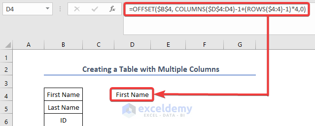
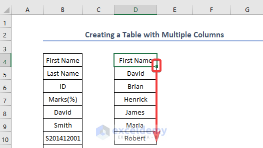
- Copy the formula down using the Fill Handle icon to cell D10.
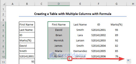
- Copy the formula right to cell G10 in a similar way.
- Select a cell in the data and press Ctrl + T. This will open a little window named Create Table.
- Mark the My Table has headers checkbox and press OK.
You’ll get a notification box.
- Hit the Yes button.

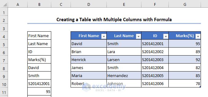
Here’s the output.
Formula Explanation:
In this part, we will break down the following formula we have used above.
=OFFSET($B$4, COLUMNS($D$4:D4)-1+(ROWS($4:4)-1)*4,0)
- (ROWS($4:4)-1)*4
The ROWS function returns the number of total rows in $4:4 range, and it’s 1. If it would be $4:6, the function would return 3.
Output: 0
- COLUMNS($D$4:D4)-1+(ROWS($4:4)-1)*4
The COLUMNS function works in a similar manner.
Output: 0
- OFFSET($B$4, COLUMNS($D$4:D4)-1+(ROWS($4:4)-1)*4,0)
Here, we specify the arguments of the OFFSET function, so the formula becomes OFFSET($B$4, 0,0). It means OFFSET will advance to 0 rows and 0 columns forward from cell B4, and return that cell value. As you copy the formula rightward and downward, the relative references inside the formula change accordingly, and the OFFSET function will return corresponding cell values.
Read More: How to Create a Table with Merged Cells in Excel
Method 2 – Use Power Query in Excel to Create a Table with Multiple Columns
Let’s assume that the column contains lots of blanks and unwanted characters.
Steps:
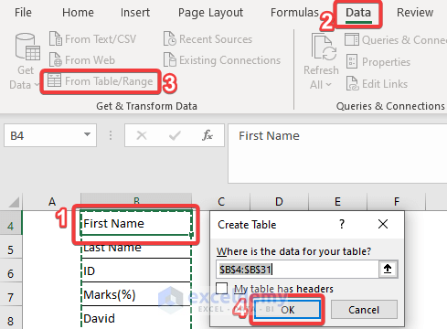
- Select any cell in the column.
- From the Data ribbon, select From Table/Range.
- A small window will be opened. Ensure the My table has headers checkbox is unmarked.
- Press OK.
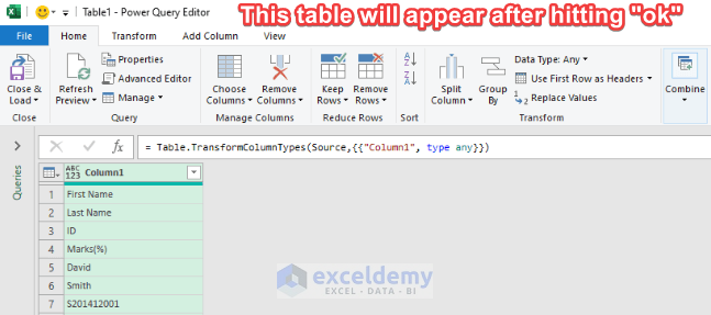
It will bring up the power query editor.
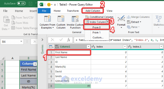
- Under the Add Column section, go to the Index Column option and click on the drop-down.
- Select From 0.
- Repeat the process to create a third column.
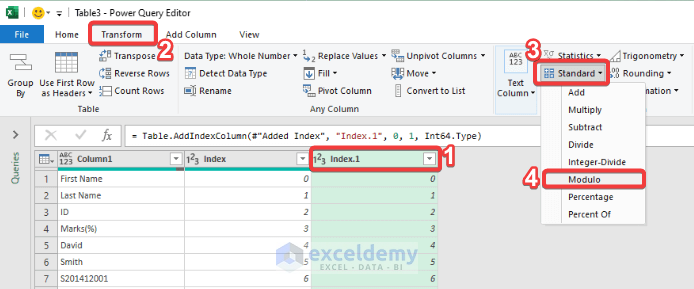
- We need to divide the third column by 4 (as we are working with 4 columns). Select that column.
- Click Transform, then go to Standard and use Modulo.
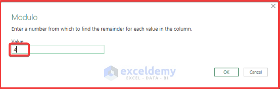
- Enter the number of columns, in this case 4.
- Hit OK.
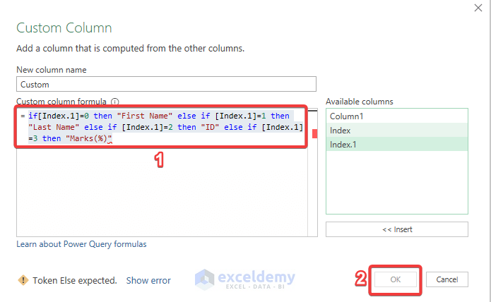
- Go to Add Column and select Custom Column.
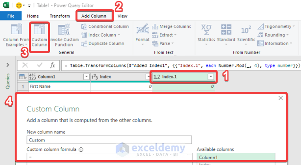
- Enter the following in the Custom column formula box.
if[Index.1]=0 then "First Name" else if [Index.1]=1 then "Last Name" else if [Index.1]=2 then "ID" else "Marks(%)"- Hit OK.
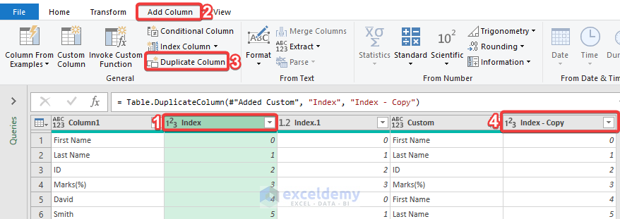
- We need to duplicate the second column (‘1’ in the image) to get the fifth column (‘4’ in the image). With the column selected, go to Add Column and select Duplicate Column.
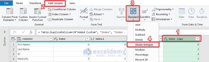
- We will divide the 5th column by column number 4. Go to the Add a Column tab and from the Standard option choose Divide (integer).
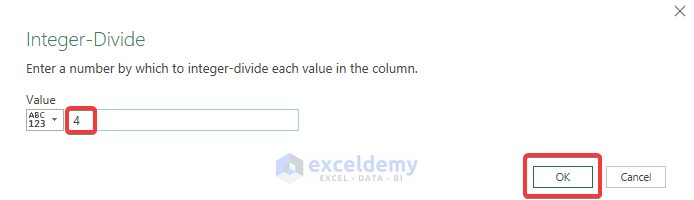
- Enter 4 for the column number. And hit OK.
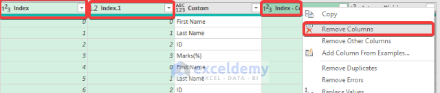
- Remove the 2nd, 3rd, and 5th columns will be removed as they are just for calculations.
- In the Home ribbon, go to Remove Rows and click Remove Top Rows.
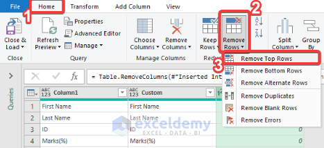
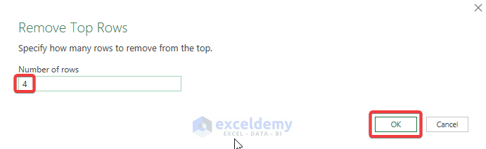
- Enter 4 in the pop-up Remove Top Rows box and hit OK.
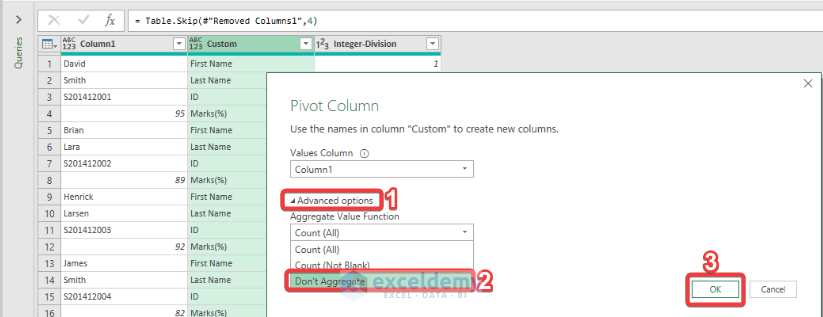
- Select the middle column and go to Transform, then go to Pivot Column.
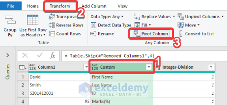
- In the Advance Options, select Don’t Aggregate.
- Click OK.
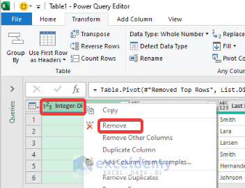
- Right-click on the header for the first column and select Remove.
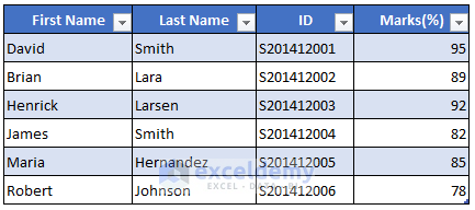
- The expected table shown below should appear.

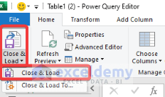
- Load the table by hitting Close & Load under the Home tab.
- This table will be loaded into the worksheet.
Read More: Create Table in Excel Using Shortcut
Download the Practice Workbook
Related Articles
- Create a Table in Excel Based on Cell Value
- How to Create a Table with Existing Data in Excel
- How to Create a Table Without Data in Excel
- How to Make a Table in Excel with Lines
- How to Create a Table with Subcategories in Excel
- How to Add New Row Automatically in an Excel Table
<< Go Back to Excel Table | Learn Excel
Get FREE Advanced Excel Exercises with Solutions!
