Latest Posts From Al Ikram Amit

Download the Practice Workbook EMI Calculator.xlsx Overview of the EMI Calculation The Equated Monthly Installment, or EMI, is payment for ...
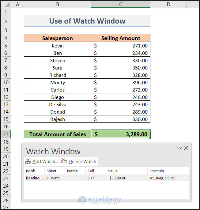
Method 1 - Using Watch Window to Create Floating Cells To make particular info available all the time while scrolling through big data in Excel, add a ...

This tutorial will show you how to create a meter chart in Excel. Learning how to create a meter chart in Excel can help you monitor your data in an organized ...

In this tutorial, we will show how to insert and customize markers in Excel. We will also show how to add pictures as data markers and how to add markers in ...

Download the Practice Workbook Using Power Map in Excel.xlsx How to Enable the Power Map Add-in in Excel Go to File and select Options. An ...
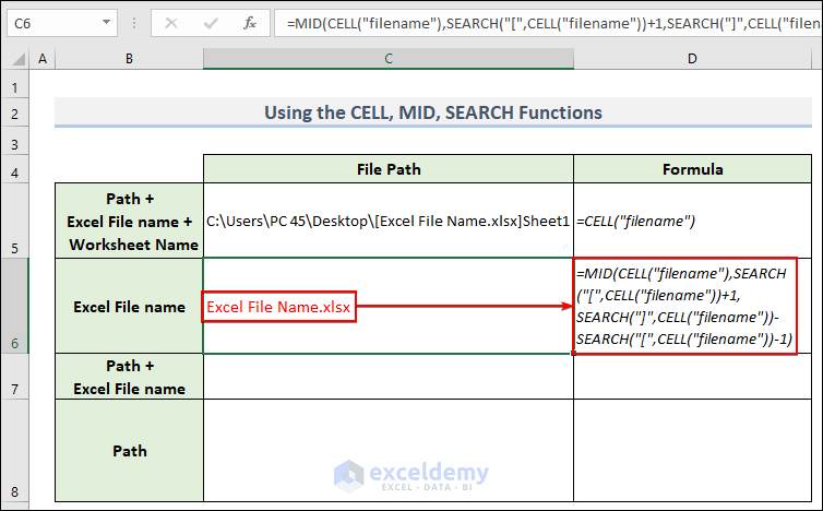
In this article, we explore the different ways of getting the Excel file name directly from Excel. Often, mastering a variety of features and functions is ...

This tutorial will show you how to change the Chart Style in Excel. Learning how to change the chart style can help your charts look better overall. Excel ...

This article will explain the importance of using visible cells only, how to use them effectively, and how it affects your Excel calculation. Excel is a strong ...

This blog post will walk you through the process of swapping individual cells, rows, or columns, highlight its importance in data management, and offer helpful ...

In this blog post, we'll delve into the Excel world of stocks and examine some of the valuable features found in the Stocks ribbon, which is located under the ...

The house estimation allows us to create a reasonable budget, which will eventually lead to a proper path toward managing the construction of a house without ...

Method 1 - Using a Color Combination Based on Values Steps: Choose the set of cells containing the values you want to make a good color combination. We ...

Example 1 - VBA Worksheet Change Event Based on the Continuous Multiple Cells Steps: In Excel, you can open the VBA Editor by pressing "Alt + F11" or by ...
Method 1 - Directly Setting One Cell Value in Another Sheet Steps: Press Alt + F11 to open the VBA Macro. Click on the Insert. Select the Module. ...

In the article, titled VBA Evaluate Array Formula, we'll look at three effective ways to use VBA's Evaluate function to efficiently manipulate data in Excel. ...
- 1
- 2
- 3
- …
- 6
- Next Page »
See Our Reviews at


Dear NU,
Thank you for your engagement with our content. If you’re using the provided code, please ensure it aligns with your specific dataset and pivot table configuration. To assist you further, could you kindly provide the specific dataset you are working with? Your dataset will be invaluable in ensuring we accurately address your query.
Alternatively, you may also try the following modified code, which aims to rectify the issue:
Note: This modified code includes a boolean variable
foundto track whether a matching item is found infiltvalues.If no match is found,
pitm.Visibleis set toFalseto hide the item.If a match is found,
pitm.Visibleis set toTrueto show the item.We appreciate your cooperation and look forward to resolving this matter promptly.
Best regards,
Al Ikram Amit
ExcelDemy
Hi Gracie,
I see you encountered an issue with the formula provided earlier. The circular reference error occurs because the formula is attempting to reference the same range (M$4:M4) it’s currently located in, which creates a circular dependency.
To address this, I recommend using a VBA solution to find the top 5 most frequent numbers and their frequencies in the range M4:N9. VBA allows us to perform more complex calculations and avoid circular reference problems.
To use this VBA code, press Alt+F11 to open the VBA editor in Excel. Then, click Insert>> Module to insert a new module. Copy and paste the code into the module.
This VBA code will find the top 5 most frequent numbers in the data range E2:I57 and display them in the range M4:M9 and their corresponding frequencies in N4:N9. Remember to adjust the sheet name(We have used the sheet name “
Sheet1“) and range references in the code are matched with your data.If you have any further questions or need more assistance, feel free to ask.
Best regards,
Al Ikram Amit
Team ExcelDemy
Dear KEN,
Thank you for your question. If your data is spread across columns A, B, C, and D, you can still work out the 5 most frequent numbers and their frequencies using Excel formulas. Here’s a step-by-step approach:
=IFERROR(MODE(IF(COUNTIF(F$4:F4,$A$5:$D$23)={0},$A$5:$A$23)),"")=COUNTIF($A$5:$D$23,F5)I hope this helps! If you have any further questions, feel free to ask.
Best regards
Al Ikram Amit
Team ExcelDemy
Dear KUNAR,
Thank you for your comment. It seems that you are encountering an issue with the “Edit Credentials” prompt in Excel. This prompt usually appears when there is a need to specify the connection details or credentials for accessing external data sources. Make sure you have marked the box in the Privacy Levels window.
If you are still experiencing issues or have any further questions, please let me know, and I’ll be happy to assist you further.
Best regards
Al Ikram Amit
Team ExcelDemy
Dear ASKA,
Thank you for bringing the mistake to our attention. We apologize for the error in my previous response. You are correct, the name of the table in Excel should be “MyTable,” not “Table1”.
I apologize for any confusion caused by the incorrect information. If you have any further questions or need assistance with any other topics, please feel free to ask.
Best regards,
Al Ikram Amit
Team ExcelDemy
Dear ATEEB,
Thank you for reaching out. I’m here to help you with your Excel queries. Regarding your questions about creating alerts and blinking or flashing text in Excel, please find the answers below:
How to create a pop-up alert in Excel
To create a pop-up alert in Excel, you can use a combination of VBA (Visual Basic for Applications) code and Excel’s event triggers. Here’s an example code snippet that you can use:
Copy and paste this code into the sheet module (e.g., press Alt+F11 to open the Visual Basic Editor, find the relevant sheet in the Project Explorer, and double-click on it to open its code window). Replace “$A$1” with the cell reference that should trigger the alert.
Customize the alert message within the MsgBox function to suit your requirements. After changing cell A1, the alert message will appear.
How to blink or flash text of a specific cell in Excel
Excel does not provide a built-in feature to directly make text blink or flash. However, you can achieve a similar effect by using VBA code to toggle the cell’s font color.
In the following code, we’re toggling the font color between red and black for the specified cell (in this case, cell A1). Adjust the cell reference and customize the number of blinks and the timing (in seconds) to meet your specific requirements.
Here’s an example code snippet that demonstrates this:
Dear Fremont,
Thank you for sharing your experience and the variation you encountered regarding frozen panes in Excel. Your observation highlights an important aspect of freezing panes, particularly when not all initial rows or columns are visible during the freezing process. In such cases, the unfrozen rows or columns that are not displayed can become inaccessible for scrolling.
Your solution to unfreeze everything is indeed a valid approach to overcome this limitation. By unfreezing all rows and columns, you can regain full control and visibility of the entire worksheet, allowing for seamless scrolling and navigation.
We appreciate your input and valuable contribution to the discussion. If you have any further questions or need assistance with any other topics related to Excel, please feel free to ask.
Best regards,
Al Ikram Amit
Team ExcelDemy
Dear A,
Are you using mobile version of Google drive?
The Settings option in the latest web version of Google drive is as it is in this post. It will be better if you can send a screenshot to our forum (here is our forum link: https://exceldemy.com/forum/). So we can understand what problem you are facing.
Regards.
Al Ikram Amit
Team ExcelDemy
Hello KP MENON,
Greetings! We appreciate you contacting us and commenting on our Excel blog post with your query. If the VBA code is not working properly in Office 365, you can provide the Excel file here. We will try our best to give the updated version of that VBA code compatible with Office 365. As ExcelDemy is currently providing the best solutions of Excel related problems, feel free to provide your problems in the blogpost.
Moreover, in the following section, we have provided some troubleshooting options:
You might need to give more information about the VBA code and the events that preceded the error to troubleshoot the specific error more thoroughly. Reviewing the specific line of code where the error appears can also shed light on where the problem originated.
Regards
Al Ikram Amit
Team ExcelDemy
Hello CALEB,
Greetings! We appreciate you contacting us and commenting on our Excel blog post with your query. We appreciate your interest and are available to help. Enter the following VBA code in your module and correct the range in that code. Hopefully, this will implement the “Enter” function key in Excel which means the code will activate the next blank cell.
The result will be like this.
If you enter =CHAR(13) in cell A1 and =CODE128(A1) in cell B1 in Excel, the following will happen:
I’ll be pleased to help you further if you can give me more information or a sample of your Excel sheet if the issue continues.
Regards
Al Ikram Amit
Team ExcelDemy
Hello SUERINA JUILINA,
Greetings! We appreciate you contacting us and leaving a comment on our Excel blog post with your query. We appreciate your interest and are available to help.
There are lackings in describing your particular problem. However here is the VBA code that probably can solve your particular problem:
Finally, “Page 2 of 2” is shown as a Page Number like in the following image:
I’ll be pleased to help you further if you can give me more information or a sample of your Excel sheet if the issue continues.
Regards
Al Ikram Amit
Team ExcelDemy
Hello MAHIN,
Greetings! We appreciate you contacting us and leaving a comment on our Excel blog post with your query. We appreciate your interest and are available to help.
First of all, you have inserted a leading zero by any of the following means:
Now, there could be a few reasons why the SUM function in Excel is failing to deliver any results for your data. Here are some recommendations to aid in troubleshooting the issue:
You should be able to fix the Excel SUM function returning null problem using the abovementioned techniques. I’ll be pleased to help you further if you can give me more information or a sample of your Excel sheet if the issue continues.
Regards
Al Ikram Amit
Team ExcelDemy
Hello KAZEM,
Greetings! We appreciate you contacting us and leaving a comment on our Excel blog post with your query. We appreciate your interest and are available to help.
The “subscript out of range” error frequently happens when the active sheet does not contain the table with the specified name.
Please double-check the table name you entered into the InputBox when prompted by the tName variable. Verify again that the table name corresponds to the one on your worksheet.
Additionally, make sure the table is on the active sheet and not on another sheet. The table is assumed to be present by the code in the active sheet.
You can try the following troubleshooting steps if the problem continues:
You should be able to fix the “subscript out of range” error by making sure these things are correct.
I sincerely hope you find this useful.
Regards
Al Ikram Amit
Team ExcelDemy