Sparklines Are Not Showing in Excel (6 Simple Solutions)

Here’s a sample dataset with sparklines that we’ll troubleshoot.

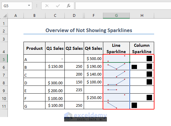
Sparklines Are Not Showing in Excel: 6 Simple Solutions

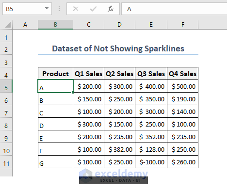
We’ll use the sample sales dataset.

Solution 1 – Upgrading Excel Version

Steps:

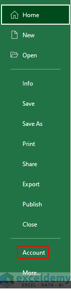
• Go to File and select Account.

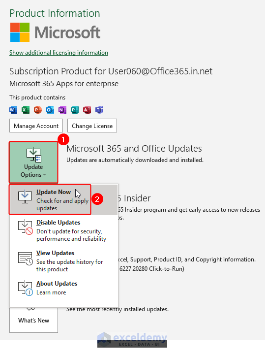
• Click on the Update Options and select Update Now. This may resolve the problem as Microsoft Excel 2010 introduced sparklines. Any versions before Excel 2010 will not show sparklines options.

Solution 2 – Choosing the Data Range and Placement of Sparklines Correctly

Steps:

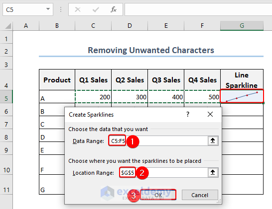
• We will go through the whole process of inserting sparklines in Excel.
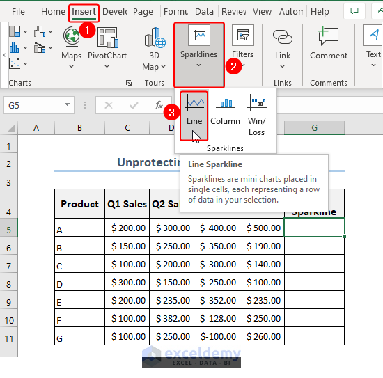
• Go to Insert and select Sparklines, then choose Line.

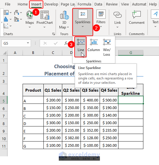
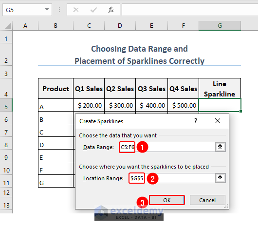
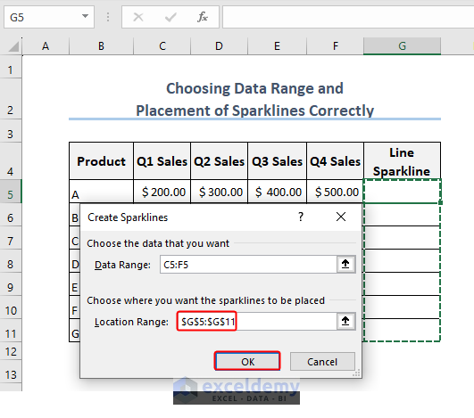
• The Create Sparklines window will appear.
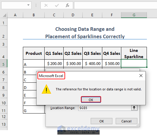
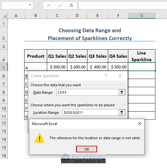
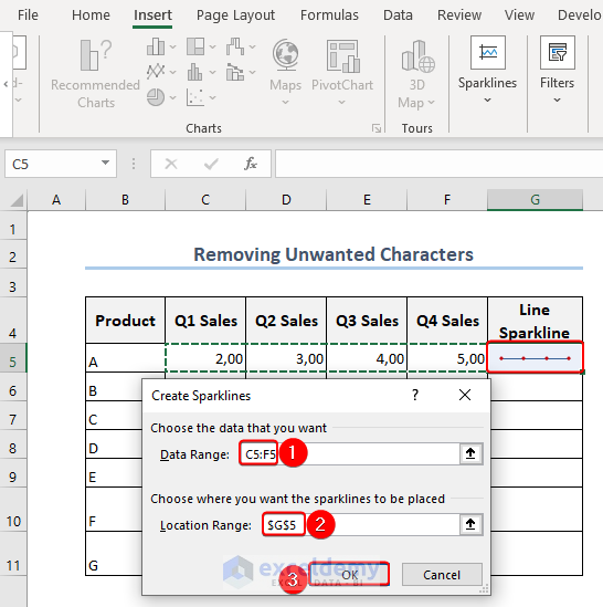
• Select Data Range: C5:F6, Location Range: $G$5 and then click OK. You’ll get an error.

• Click OK.

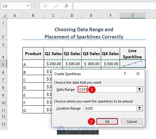
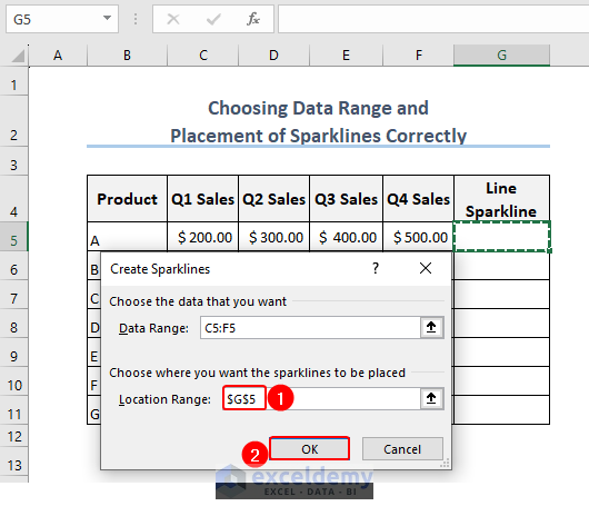
• Change Data Range: C5:F6 to Data Range: C5:F5 as the Data Range should be one dimensional.

• You can also get an error for Location Range: $G$5:$G$11.

• Click OK.

• If the result in a single cell (G5) you won’t get an error.

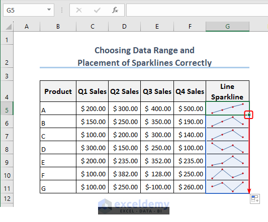
• Drag the Fill Handle down to get all Sparklines.

Solution 3 – Unprotecting the Excel Workbook

Steps:

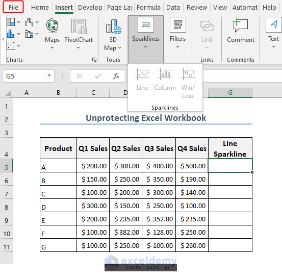
• Consider the following image where the Line under Sparklines under the Insert tab is blurred out.

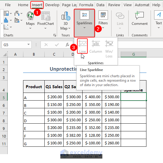
• Select File.

• Go to Review, then to Protect and select Unprotect Sheet.

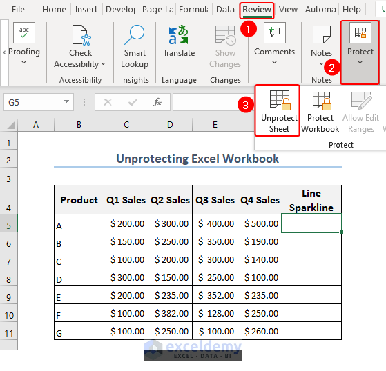
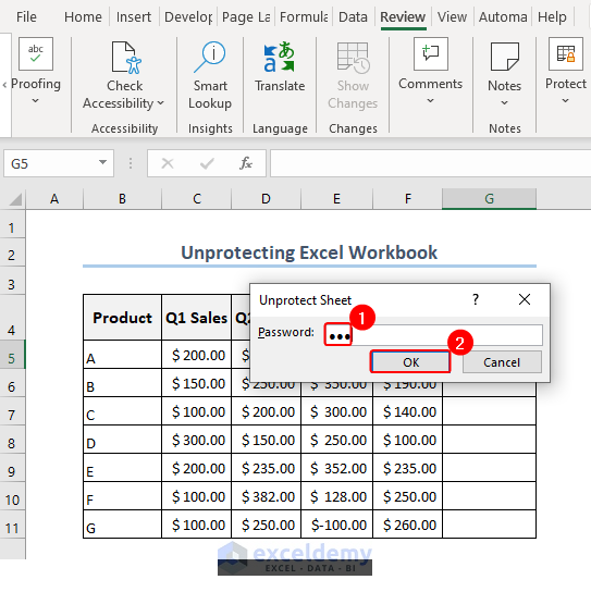
• The Unprotect Sheet window will appear.
• Insert the password and click OK.

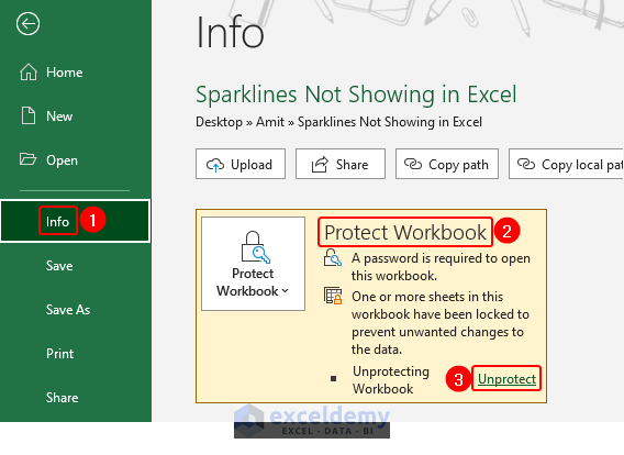
• Another way you can unprotect a sheet is by following the path: Info > Protect Workbook > Unprotect.

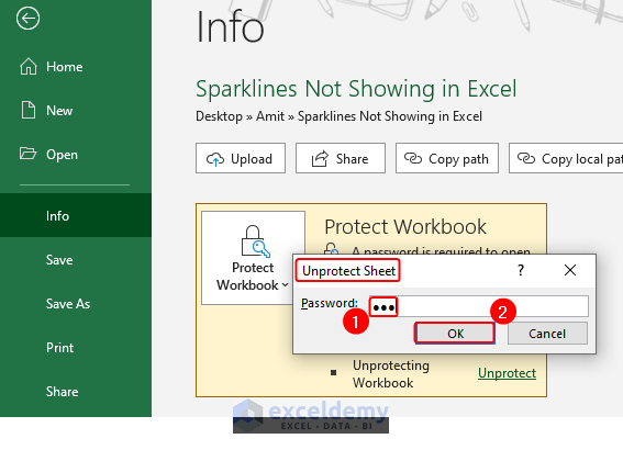
• Like the previous step, the Unprotect Sheet window will appear again and you need to insert the password and click OK.

• The Line Sparklines option is available again to use in Excel.

Solution 4 – Removing Unwanted Characters

Steps:

• In the following image, we have different data with various types of unwanted characters.

• We have different data still the Sparkline is flat. It has taken all the data as 0.

• You can replace all the unwanted characters manually if you have a small amount of data. You can go for the Replace option in Excel if you have large data.

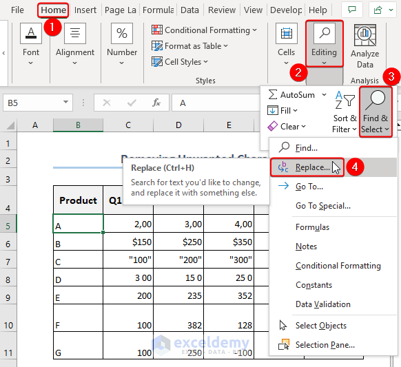
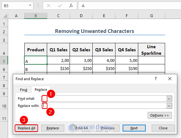
• The Find & Replace window will appear in Excel. In the Find what box insert a comma (,) and keep the Replace with box empty, and then click Replace All.

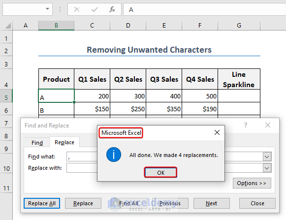
• Microsoft Excel will show a message box about all the replacements that have been done. You need to click OK.

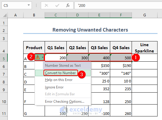
• Convert the values into numbers by pressing Smart Tags and selecting Convert to Number.

• Create the Sparklines.

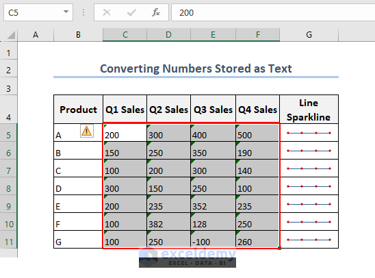
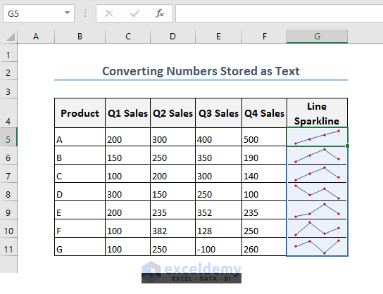
Solution 5 – Converting the Numbers Stored as Text

Steps:

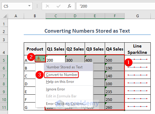
• Due to the numbers stored in Text format, all the sparklines are flat lines.

• By pressing Smart Tags and choosing to Convert to Number, you can turn them into numbers to get valid Sparklines.

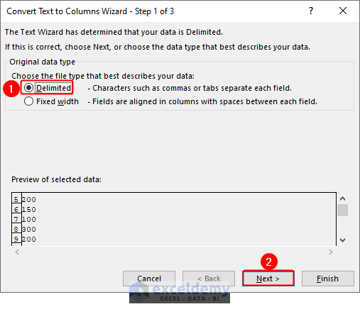
• To solve this issue, you can use Texts to Columns.

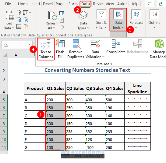
• The Convert Text to Columns Wizard- Step 1 of 3 window will appear.
• Select Delimited and click Next.

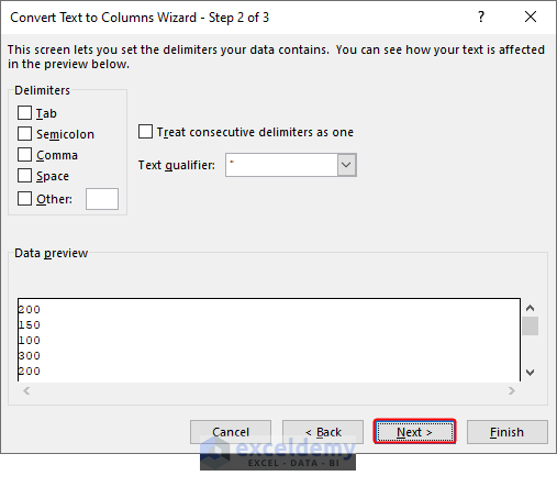
• The Convert Text to Columns Wizard- Step 2 of 3 window will appear. Click Next.

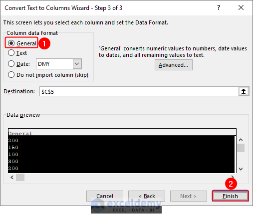
• In the Convert Text to Columns Wizard- Step 3 of 3, select Column Data Format as General and click on Finish.

• You will get the sparklines as shown in the image below.

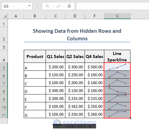
Solution 6 – Showing Data from Hidden Rows and Columns

Steps:

• In the following example, there is a hidden E column that had data on Q3 Sales. But that data is not shown in the sparklines.

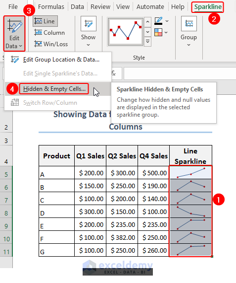
• Select the Sparklines, then go to Sparkline, choose Edit Data, and select Hidden and Empty Cells…

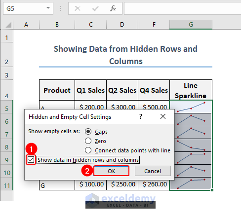
• The Hidden and Empty Cell Settings windows will appear. Mark the box Show data in hidden rows and columns and click OK.

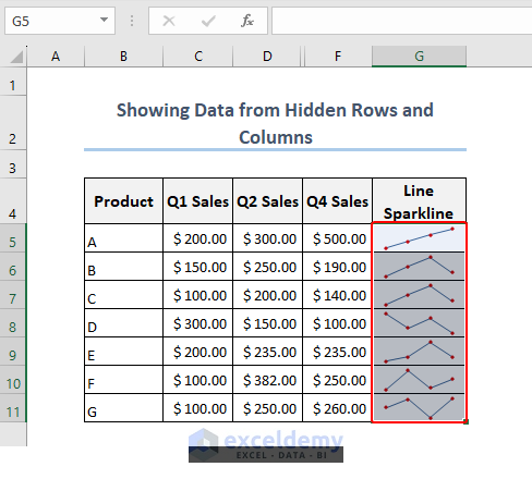
• The column E still is hidden but we get that data into the sparkline.

Download the Practice Workbook

Related Articles

• How to Change Sparkline Color in Excel 
• [Solved]: Excel Sparklines Location Reference Is Not Valid
• How to Ungroup Sparklines in Excel

<< Go Back to Excel Sparklines | Learn Excel