How to Use Sparklines in Excel (Create and Customize)

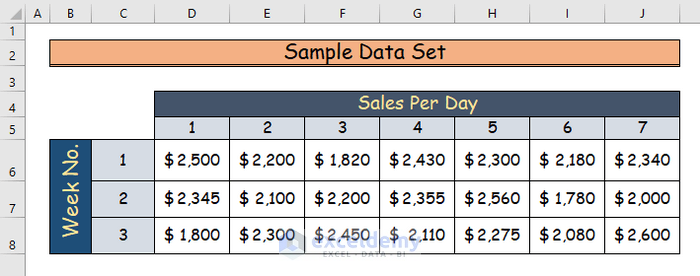
Here is a sample data set that we’ll use to create sparklines.

Step 1 – Preparing the Data Set

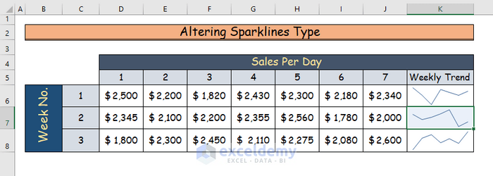
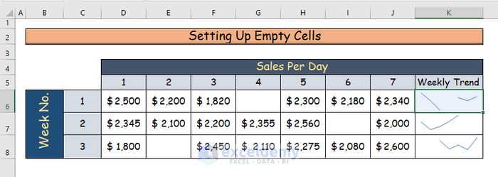
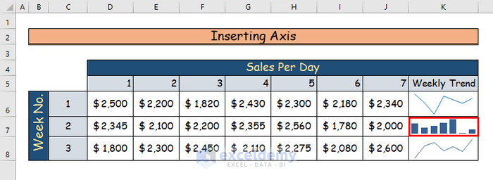
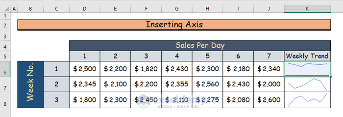
• We have the following data set, where cells D4 to J4 represent the Sales Per Day and cells C6 to C8 represent the week number.
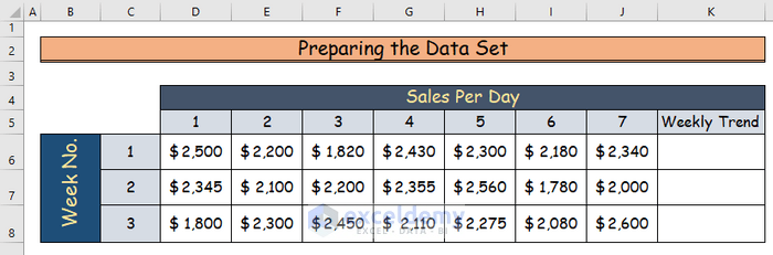
• Make three extra cells in column K to represent the Weekly Trend.

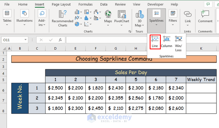
Step 2 – Choosing the Sparklines Command

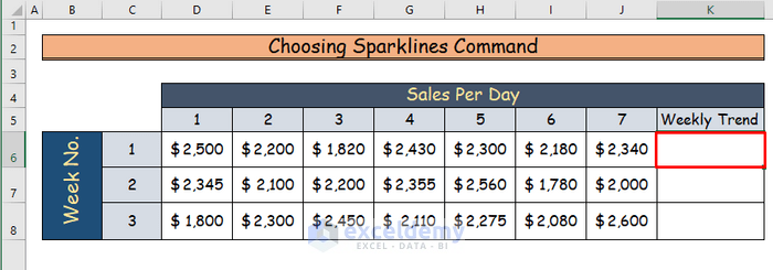
• Choose any cell from K6 to K8 in column K under the Weekly Trend header.

• Go to the Insert tab in the ribbon.
• Choose the Sparklines command from the Sparklines group.

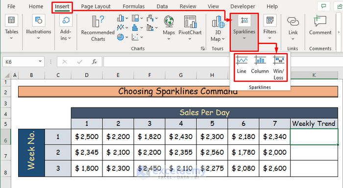
• You will see three types of sparklines. Choose one.
• We will use the Line Sparkline.

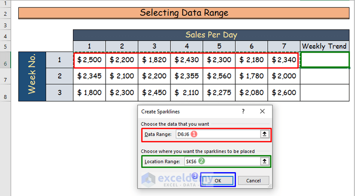
Step 3 – Selecting the Data Range

A new dialog box named “Create Sparklines” will appear.

• There are two blank spaces in the box.
• In the “Data Range” box, select the range of cells to create a sparkline. We will insert the cell range from D6 to J6.
• In the “Location Range” box, select the cell location where you want to create the sparkline.
• Press OK.

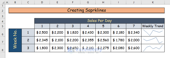
Step 4 – Creating the Sparklines

• You will see a sparkline under the Weekly Trend header in cell K6.

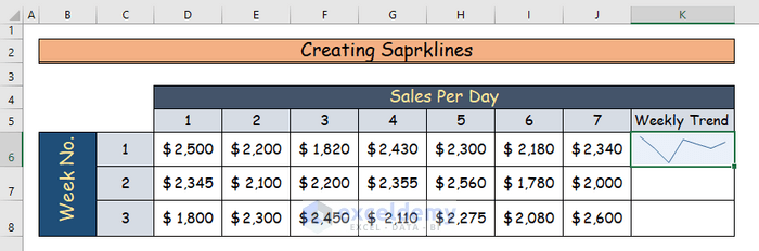
• Repeat Step 2 and Step 3 to create more sparklines in cells K7 and K8.

Read More: How to Create Column Sparklines in Excel

Formatting the Sparklines

Case 1 – Altering the Type of Sparklines

There are three types of sparklines :

1. 1. Line Sparkline
   2. Column Sparkline
   3. Win/Loss Sparkline

Steps:

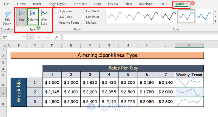
• Choose an existing sparkline that you want to alter. We selected the sparkline in cell K7.

• You will find a new tab named Sparkline in the ribbon.
• Go to Type.
• Choose the type of sparkline you want to use. We chose the Column type.

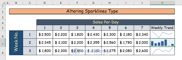
• Here’s the new sparkline in the cell K7.

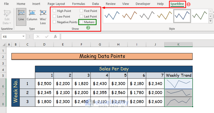
Case 2 – Making Data Points for Sparklines

Steps:

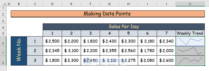
• Choose any existing sparkline. We will choose all of them.

• Go to the Sparkline tab in the ribbon.
• In the Show group, you will see many options that will mark your sparklines according to their uses. We will choose the Markers command.

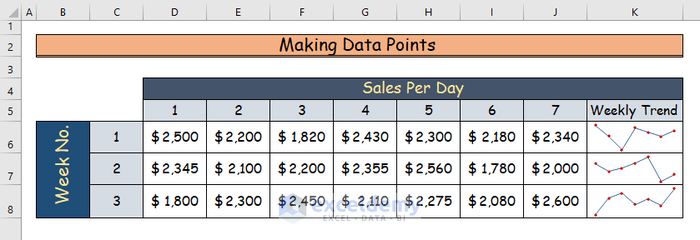
• You will see all the data points on the sparklines. This feature will help you to analyze your data quickly.

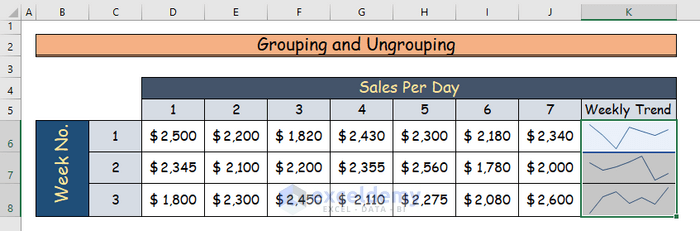
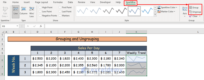
Case 3 – Grouping and Ungrouping in Sparklines

Steps:

• Select the sparklines that you want to group.

• From the Sparkline tab, go to Group. You will find two commands, Group and Ungroup.
• For grouping, choose Group.

• If you make any changes to any sparkline, you will be able to see them on other sparklines as well.

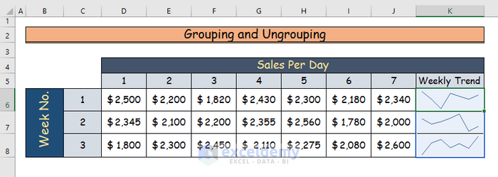
• If you make data points for only the sparkline in cell K7, then other sparklines in cells K6 and K8 will also get that.

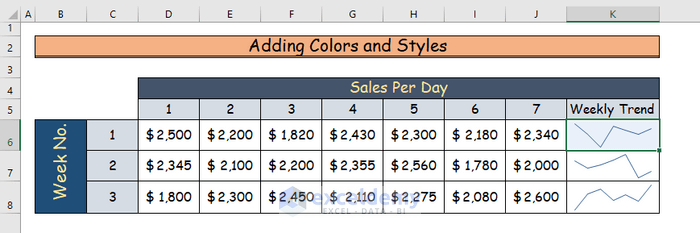
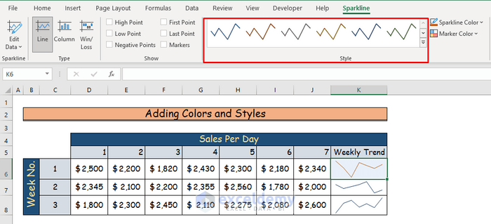
Case 4 – Adding Colors and Styles to Sparklines

Steps:

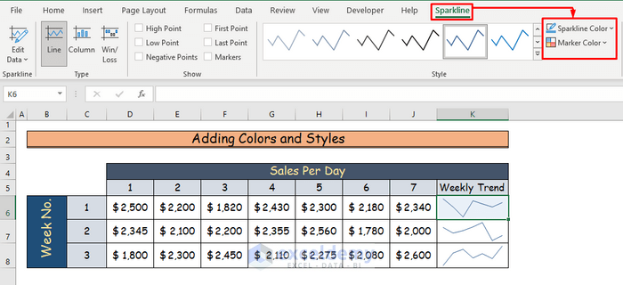
• Select the sparkline you want to change.

• From the Sparkline tab, go to the Style command. You will see two options, Sparkline Color and Marker Color.

• From Sparkline Color, you will be able to change the color of your current sparkline. Choose any color from the Theme Colors option.

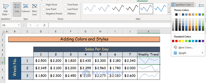
• The color of your sparkline will change.

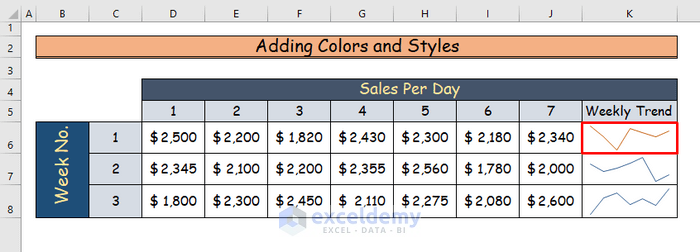
• To change the style of your sparkline, go to the Style group. Choose any style from the list.

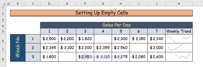
Case 5 – Setting up the Empty Data Cells for Sparklines

You may have empty data cells in your sparkline data set. You can either leave them that way or customize them in Excel.

Steps:

• Select the sparkline with empty cells.
• Go to the Sparkline tab and select the Edit Data option.
• Choose the Hidden & Empty Cells command.

• A new dialog box named “Hidden and Empty Cell Settings” will appear.
• There are three options regarding empty cells in there.
• For the first sparkline, choose the Gaps option.
  

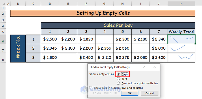
• This option will not connect the sparkline where there is a gap or empty cells.

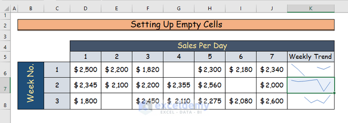
• For the second sparkline, we will choose the Zero option.

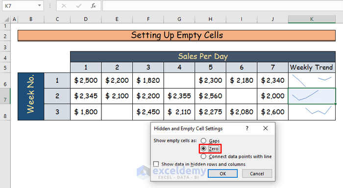
• This will assume the empty cell values as zero and will connect the sparkline.

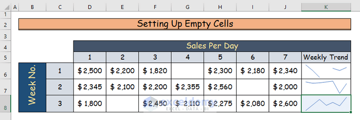
• For the third sparkline, choose the Connect data points with line command.

• This will connect data points by excluding the empty cell.

Case 6 – Inserting an Axis for Sparklines

By default, sparklines will take the lowest data point as the bottom value. You can insert an axis for the benchmark value.

Steps:

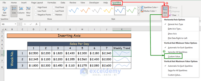
• Select the sparkline in which you want to insert the axis.
• Go to the Sparkline tab and choose the Axis option.
  
• Select the Custom Value command.
  

• A new dialog box named “Sparkline Vertical Axis Setting” will appear.
• In “Enter the minimum value for the vertical axis”, enter a value manually to start the sparkline.
• We will insert 0 as the value.

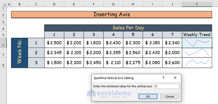
• The shape of the sparkline will change according to the minimum value.

• If you want to show the axis line, go to the Axis option again from the Sparkline tab, then choose the Show Axis command.
  

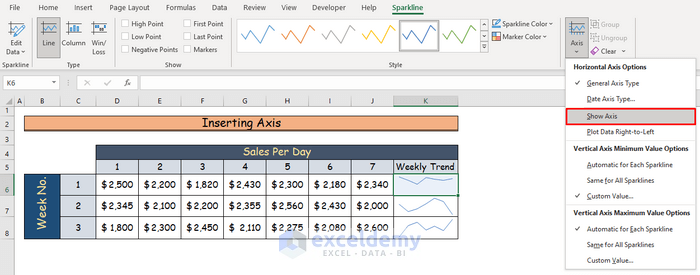
• You will see the axis under the sparkline.

Case 7 – Clearing an Existing Sparkline

Steps:

• Select the sparkline that you want to clear.
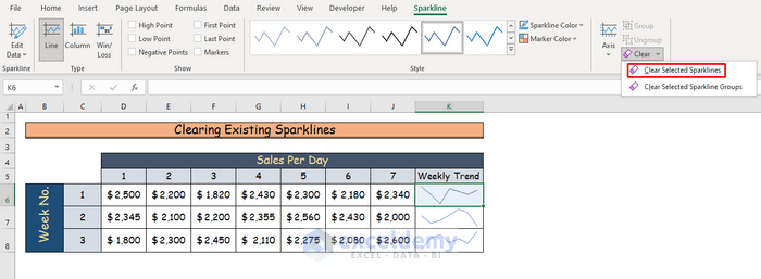
• Go to the Sparkline tab and go to the Clear option in Group.

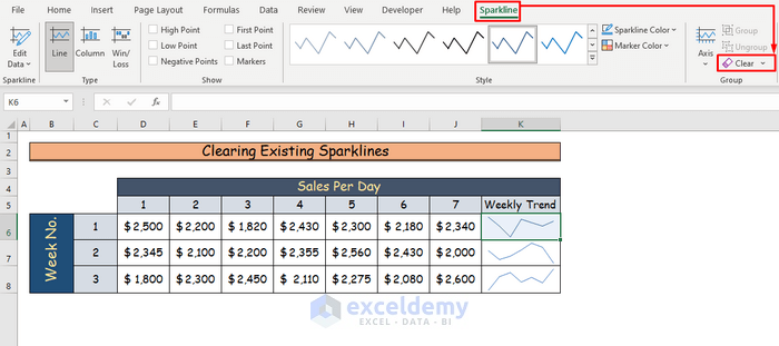
• Select the “Clear Selected Sparklines” command from the option.

• The existing sparkline will be cleared from the data set.

Download the Practice Workbook

<< Go Back to Excel Sparklines | Learn Excel