Excel Floating Cells (Create and Remove)

We’ll talk about different methods to give the spreadsheet a floating effect as we explore the idea of floating cells in Excel. Excel does not have a built-in feature for floating cells, but we will explore workarounds that can be used to get comparable results. We’ll go over strategies like floating images, text boxes, and cells as objects that offer more positioning and customization options. By mastering these methods, you can improve the visual design of your Excel worksheets and produce interactive, dynamic interfaces. Join us as we explore the potential of Excel’s floating cell feature.

Download Practice Workbook

Create and Remove Floating Cells.xlsm

How to Create Floating Cells in Excel

1. Using Watch Window to Create Floating Cells

To make particular info available all the time while scrolling through big data in Excel, you can add a watch window in Excel.
Follow the path to add a watch window: Formulas>> Formula Auditing group>> Watch Window.
The Watch Window dialog box will appear like this.

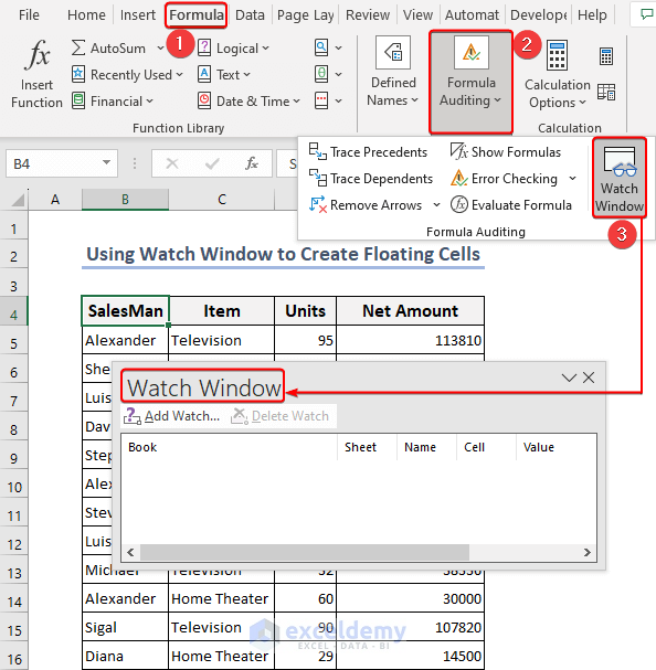
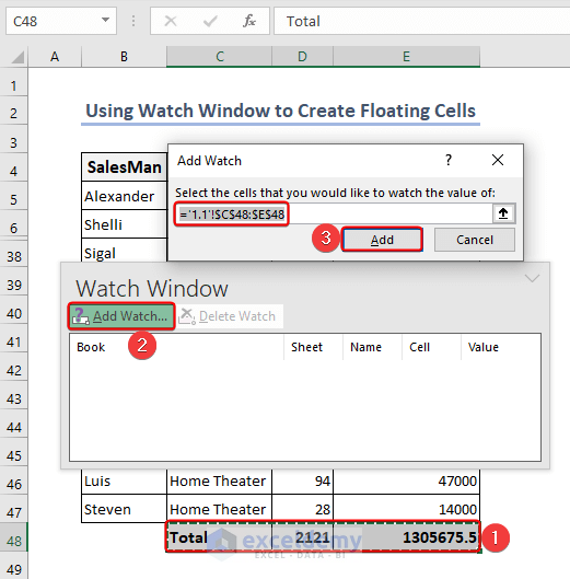
We now need to include the Watch Window. Click on Add Watch to do that.
As a result, a new dialog box titled “Add Watch” will appear. We must choose the cells we want to show in the watch window in this new dialog box. I’ve chosen C48:E48 from the “1.1” sheet in this instance. Lastly, select Add.

This watch window has the nice feature that it will automatically update even if the value of the cell changes.
Additionally, the Watch Window can be docked on top of the ribbon and will remain there even if we switch to another sheet.

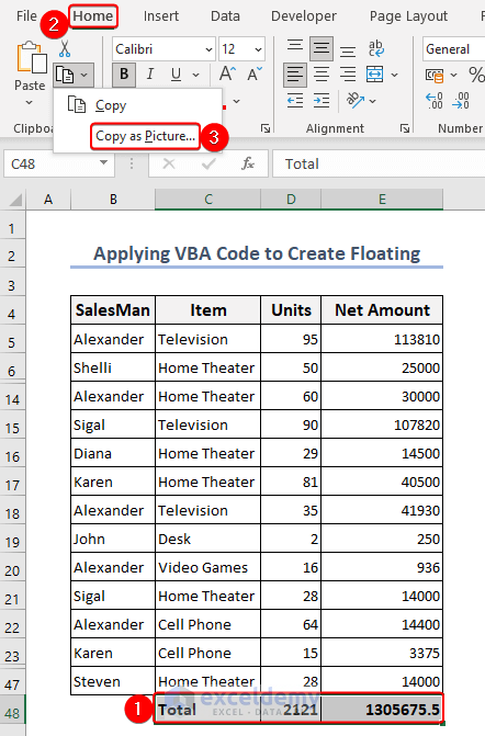
2. Applying VBA Code to Create Floating Cells

Here, the cells that we want to float on the screen will first be photographed. Select those cells first to do that. I’m choosing the range C48:E48.
Now select Copy as Picture from the Home tab.

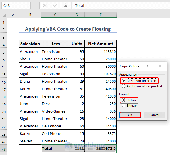
As a result, the Copy Picture dialog box will appear. To continue, click OK.

We must now paste the image into the worksheet. For the picture to be pasted, press Ctrl+V or the right button of the mouse.

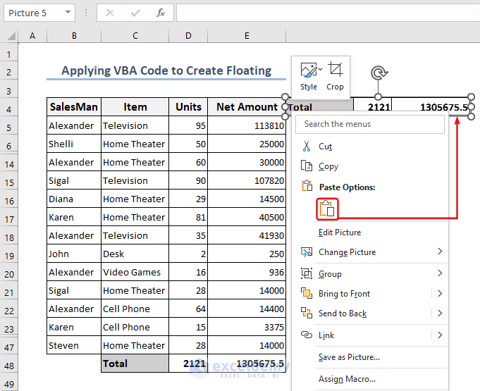
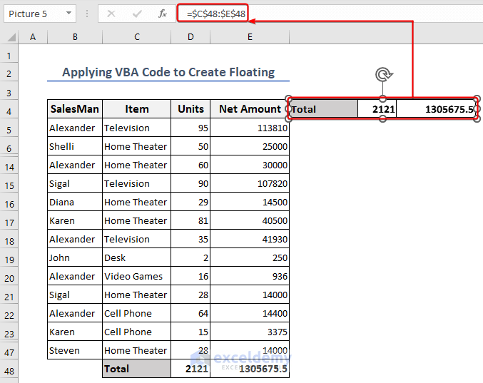
Click the pasted image once more, then go to the formula bar and type =. Select the cells that you copied as a picture right now. I have chosen C48:E48 in this case. Now hit Enter.
Consequently, this pasted image has been dynamic. This implies that any changes we make to the copied cells will also be reflected in the image.

We now need to create the code to make sure that this image is always displayed on the screen. Click Alt+F11 to launch the VBA Editor.
To access the worksheet you are working on, click its name in the window like Sheet5(1.2). After that, paste the subsequent code into the sheet window.

'Right Corner
Private Sub Worksheet_SelectionChange(ByVal A_Target As Excel.Range)
    Dim My_Picture As Object
    Dim My_Top As Double
    Dim My_Right As Double
    Dim Top_Right_Cell As Range
    '- position of the bottom right cell
    With ActiveWindow.VisibleRange
        AA_r = 4
        AA_c = .Columns.Count
        Set Top_Right_Cell = .Cells(AA_r, AA_c)
    End With
    '- Setting position of the picture
    Set My_Picture = ActiveSheet.Pictures(1)
    My_Top = Top_Right_Cell.Top + 5
    My_Right = Top_Right_Cell.Left - My_Picture.Width
    With My_Picture
        .Top = My_Top
        .Left = My_Right
    End With
End Sub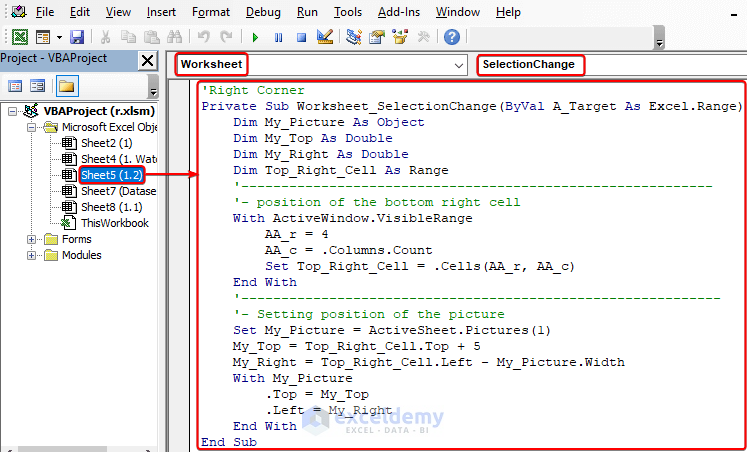

VBA Explanation

Private Sub Worksheet_SelectionChange(ByVal A_Target As Excel.Range)

In the worksheet where the code is located, this line declares a worksheet event handler that fires whenever the selection changes.

Dim My_Picture As Object

Dim My_Top As Double

Dim My_Right As Double

Dim Top_Right_Cell As Range

A variable called My_Picture is designated as an object in this line. This line specifies the double data type for the variable My_Top. This line specifies the double data type for the variable My_Right. In this line, the variable Top_Right_Cell is designated as a range object.

With ActiveWindow.VisibleRange

AA_r = 4

AA_c = .Columns.Count

Set Top_Right_Cell = .Cells(AA_r, AA_c)

End With

The VisibleRange block is used to define a range object that symbolizes the visible area of the currently active Excel window. The desired row index is then represented by setting the AA_r variable to 4. Next, the .Columns.Count function is used to assign the AA_c variable. Finally, the visible range’s cell at row AA_r and column AA_c is selected as the Top_Right_Cell range object. As a result, the code can use the visible range’s bottom-right cell as a reference and carry out operations according to its location.

Set My_Picture = ActiveSheet.Pictures(1)

My_Top = Top_Right_Cell.Top + 5

My_Right = Top_Right_Cell.Left - My_Picture.Width

The first picture object in the active sheet is assigned to the variable My_Picture using ActiveSheet.Pictures(1). The picture is then offset vertically by setting the My_Top variable to the top position of the Top_Right_Cell range object plus 5 units. Additionally, to guarantee that the image is placed to the left of the cell, the My_Right variable is set to the left position of the Top_Right_Cell range object minus the width of the My_Picture object.

With My_Picture

.Top = My_Top

.Left = My_Right

End With

The code adjusts the picture object’s vertical position within the With My_Picture block by setting the Top property to the value contained in the My_Top variable. Similarly to this, the Left property’s value, which establishes its horizontal position, is set to the value kept in the My_Right variable.

End Sub

In VBA code, the “End Sub” statement is used to indicate the conclusion of a subroutine or procedure.

Press Ctrl+S to save the code now. Now go to the primary worksheet after that. You will now notice that the image will appear next to your selection even if you scroll down and choose a cell.

How to Create Floating Comment

1. Using the Review Tab to Create a Floating Comment

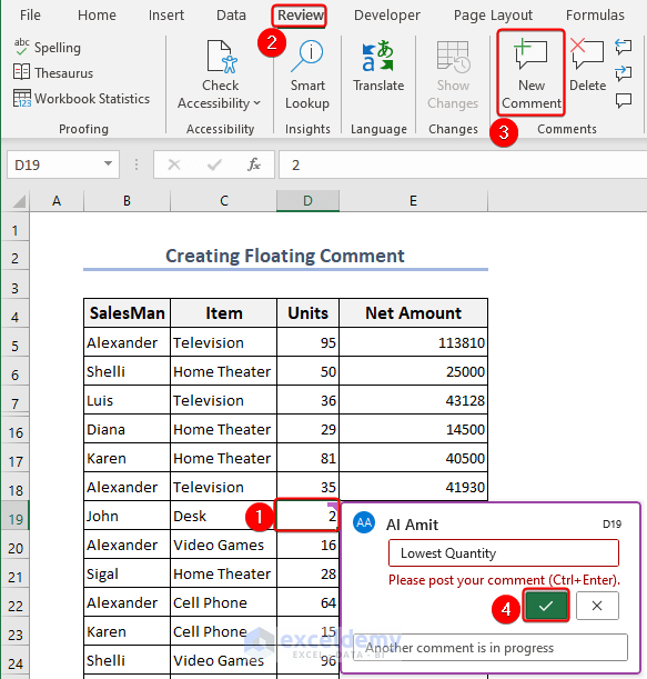
Select cell D19 first. Navigate to the Review tab next. Next, select “New Comment” from the menu.

2. Using VBA to Add Floating Comment

Start by selecting the workbook’s active sheet.
Go to the Developer tab.
Afterward, select Visual Basic.
Choose Insert, then Module after that—in the Module Box copy the following code and paste it there.

Sub addFloatingComment()
Worksheets("2.2").Cells(19, 4) _
.AddComment ("Lowest Quantity")
End Sub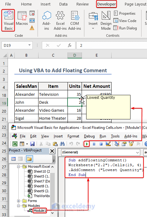

How to Create Floating Text Box in Excel

Start by selecting the Insert tab from the Ribbon.
After that, select Text Box from the Text group. Draw the text box you want. The following text box was made by us in this instance.
Click on the freshly created text box after that.
Next, type equal (=) in the formula bar.
Then, select the cell that you want to display in the text box by clicking it. We chose cell $C$48 in this instance.
This is how your final formula will look:

=$C$48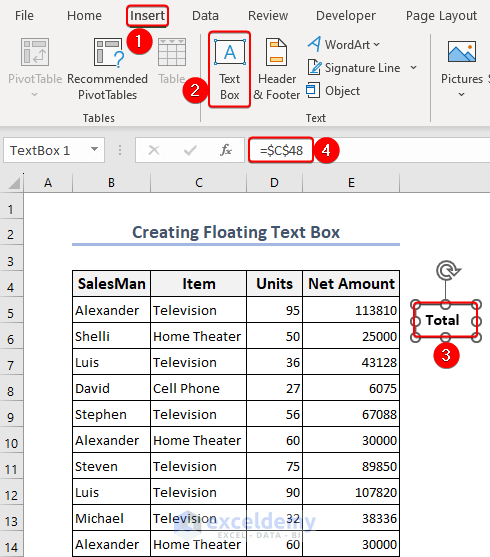

Similarly, we have added another text box in Excel like in the previous step.
Then select the Shape Format tab from the Ribbon.
Next, select the Group option from the Arrange group by clicking.
Finally, select Group from the drop-down menu.

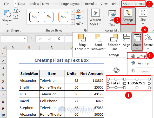
After grouping the text boxes, you can move them freely over the worksheet, like the following.

How to Create a Floating Table in Excel

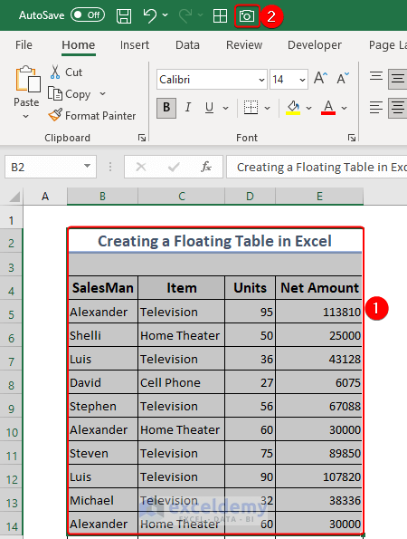
1. Creating a Floating Table Using a Camera Tool

To create a floating table using Camera, you need to bring that option in the Quick Access Toolbar. So follow the path to bring that Camera option: Customize Quick Access Toolbar>> Excel Options Window>> Quick Access Toolbar>> Choose commands from: All Commands>> find Camera option>> click on Add>> Lastly click on OK.

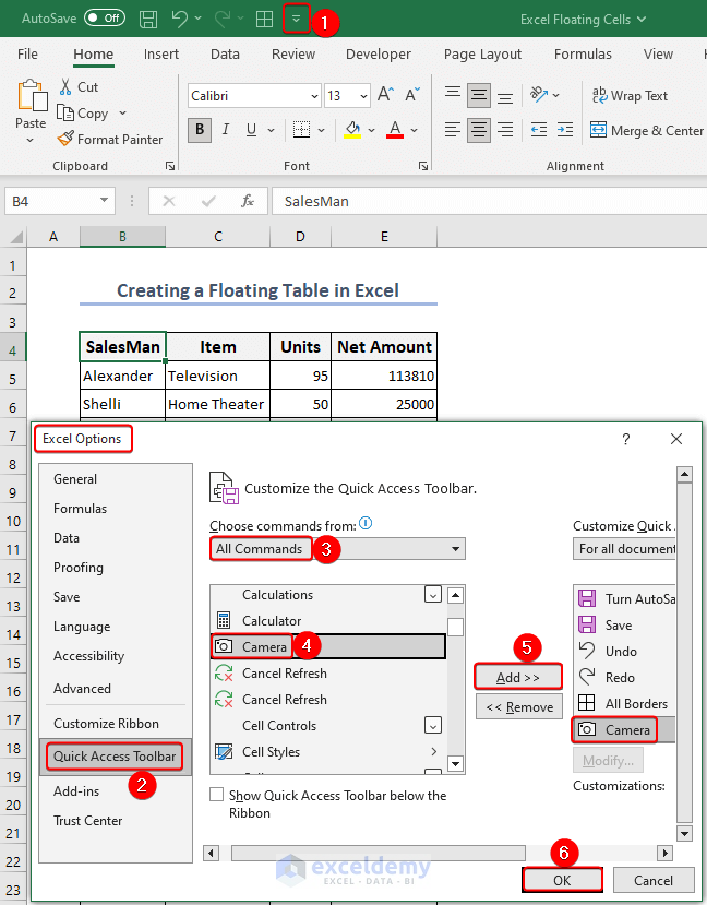
Now you will have the Camera option in the Quick Access Toolbar. First, select the table you want to float, and then click on the Camera.

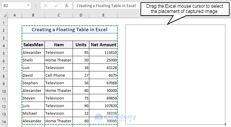
To choose where the captured image will be placed, drag the Excel mouse cursor.

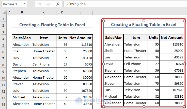
Here is the final image of a floating table in Excel. One of the most intriguing facts is that, if you change any one of the cells in your table, the data will automatically update itself in the floating table.

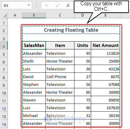
2. Creating a Floating Table Using Paste Picture

Copy your preferred table by pressing Ctrl+C.

Paste it by clicking on the right button of the mouse and then Paste Special>> Picture(U).

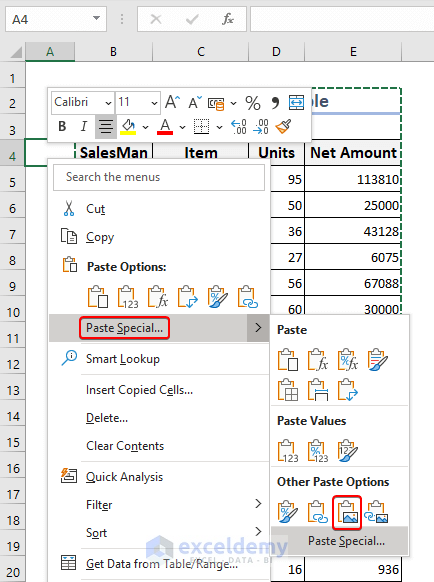
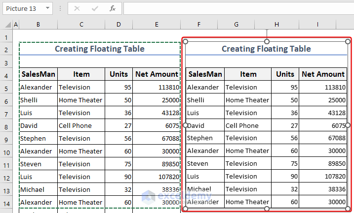
The following image shows the result of the pasted picture.

To make the table float in Excel, copy the following code and paste it into the corresponding sheet’s module

'Right Corner
Private Sub Worksheet_SelectionChange(ByVal A_Target As Excel.Range)
    Dim My_Picture As Object
    Dim My_Top As Double
    Dim My_Right As Double
    Dim Top_Right_Cell As Range
    '- position of the bottom right cell
    With ActiveWindow.VisibleRange
        AA_r = 4
        AA_c = .Columns.Count
        Set Top_Right_Cell = .Cells(AA_r, AA_c)
    End With
    '- Setting position of the picture
    Set My_Picture = ActiveSheet.Pictures(1)
    My_Top = Top_Right_Cell.Top + 5
    My_Right = Top_Right_Cell.Left - My_Picture.Width
    With My_Picture
        .Top = My_Top
        .Left = My_Right
    End With
End Sub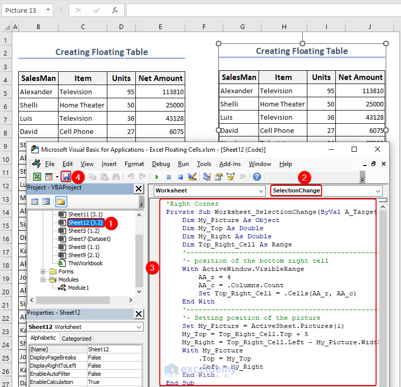

After saving the VBA code in the sheet’s module, you have made the picture available by clicking anywhere in the worksheet and the table will be beside your selection.

How to Remove Floating Objects

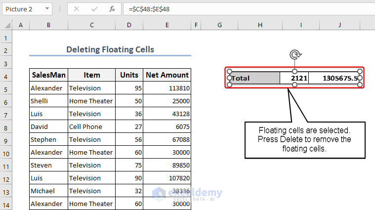
1. Using Go To Feature to Delete Floating Table

To find floating objects, press F5. Go To window will appear as a result. Press on Special.

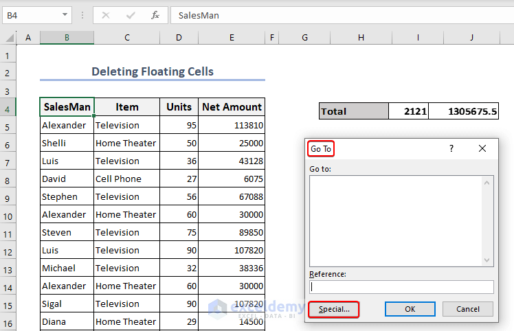
In the Go To Special window, mark the Object and click OK.

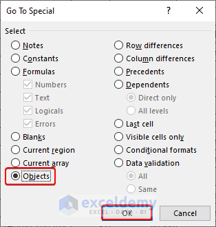
Now press Delete to remove the selected Object.

2. Applying VBA Code to Delete Floating Text Box

Choose Visual Basic first from the Developer tab. After that, a window for Microsoft Visual Basic for Applications will appear.
Write the VBA code by selecting Module from the Insert tab at this time. A new module will now open, and this is where we need to enter the code.
Therefore, add the following code to the module:

Sub DeleteAllTextBoxes()
ActiveSheet.TextBoxes.Delete
End Sub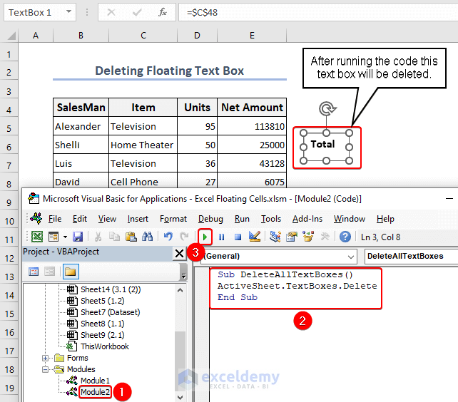

Things to Remember

Understanding Floating Cells: In Excel, cells that are positioned on top of other cells are known as floating cells. These cells are typically used for data labels or annotations.
Adjusting Floating Cell Position: A floating cell can be moved by clicking and dragging it to the desired location. By clicking and dragging the corner handles, you can resize the floating cell.
Working with Floating Cell Text: By double-clicking a floating cell, you can edit the text or data contained therein. The editing text box will then be activated.
Saving and Sharing Worksheets with Floating Cells: When you save a worksheet that has floating cells, the data in the worksheet and the floating cells will both be saved. But be aware that when opened on a different computer with a different screen configuration, floating cells might not keep their precise position and formatting.

Frequently Asked Questions (FAQs)

1. Is it possible to create floating cells inside the Excel grid system?

Answer: No, there isn’t a built-in feature in Excel that allows you to create floating cells within the grid. Since they are intended to be a part of the grid, cells cannot be placed or moved at will.

2. In Excel, how do I create a floating effect?

Answer: Although floating cells cannot be made, there are other ways to create the illusion of floating by positioning and altering elements on the worksheet, text boxes, shapes, and floating images.

3. Can I move cells around freely in Excel like other objects?

Answer: The answer is no; in Excel, cells cannot be moved freely within the grid. The only things that can be moved and positioned independently are objects like text boxes, pictures, and shapes.

Excel Floating Cells: Knowledge Hub

Conclusion

Thus far, Excel’s built-in feature does not allow for the creation of floating cells. Alternative techniques, such as floating images, text boxes, shapes, or form controls, can be used to create the floating effect. Although these techniques use manual formatting and positioning to create unique layouts, they are not the same as truly floating cells within the grid system. Consider using additional tools like Microsoft Access or specialized data visualization software for floating capabilities that are more advanced.

<< Go Back to Data Visualisation in Excel | Learn Excel

Get FREE Advanced Excel Exercises with Solutions!