Method 1 – Using the INDEX and ROW Functions
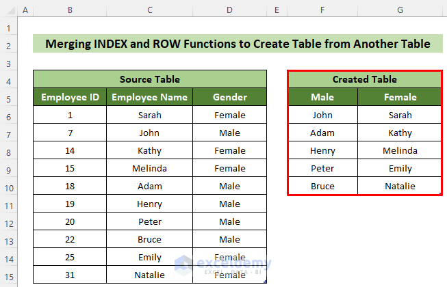
We’ll use a table named Source_table with three columns named Employee ID, Employee Name, and Gender.
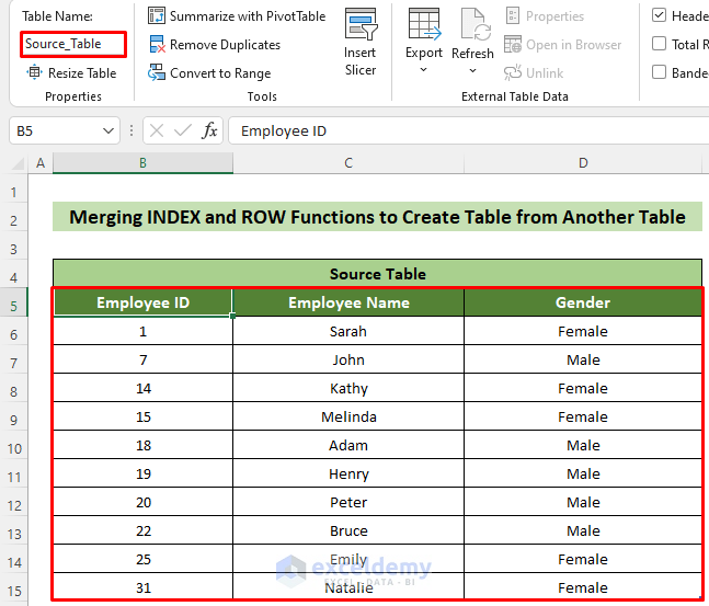
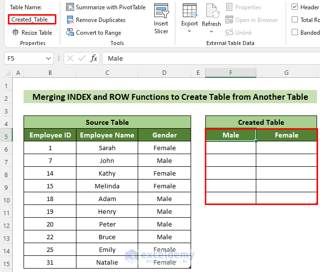
We need to create another table named Created_Table from the table above, where there will be two columns named Male and Female and the employee names will be inserted accordingly.
We can do this by merging the IFERROR, INDEX, SMALL, IF and ROW functions.
Steps
- Click on cell F5 and create a new table named Created_Table with the necessary column headings.
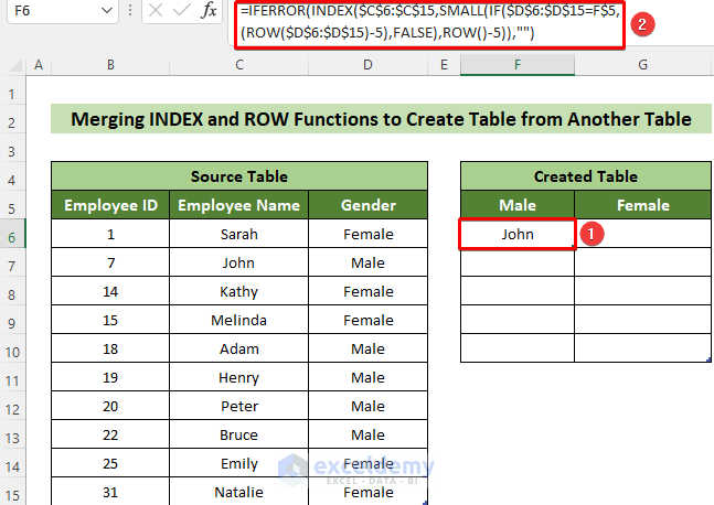
- Click on cell F6 and enter the following formula:
=IFERROR(INDEX($C$6:$C$15,SMALL(IF($D$6:$D$15=F$5,(ROW($D$6:$D$15)-5),FALSE),ROW()-5)),"")-
- This formula retrieves the names of male employees based on the dataset.
- Press Enter to get the name of the first male employee.
- Drag the fill handle rightward and downward to complete the table.
- The subtraction of 5 from the ROW function accounts for the formula being in the 6th row and looking up criteria from the 6th row. Adjust this value as needed.
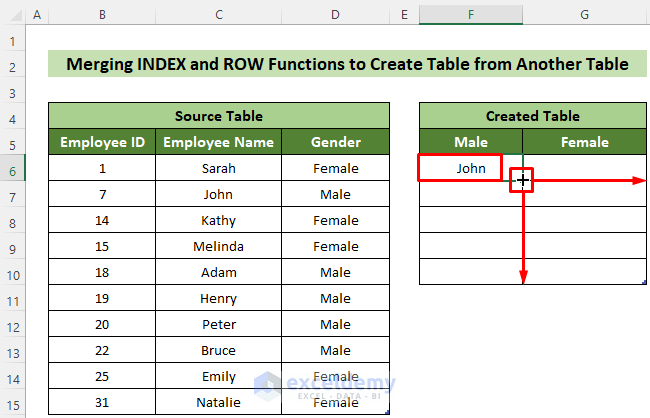
- We’ll now have a table created from another table based on our desired criteria.
Read More: How to Create Table from Another Table in Excel
Method 2 – Using VLOOKUP and COLUMN Functions
We’ll use a dataset of employees with two tables. Table1 has 2 columns: Employee ID and Employee Name. Table2 contains two columns named Employee ID and Joining Date.
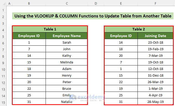
Now, we need to update Table1 by inserting the joining dates column from Table2.
We can use the VLOOKUP, IFERROR and COLUMN functions together to do this.
Steps
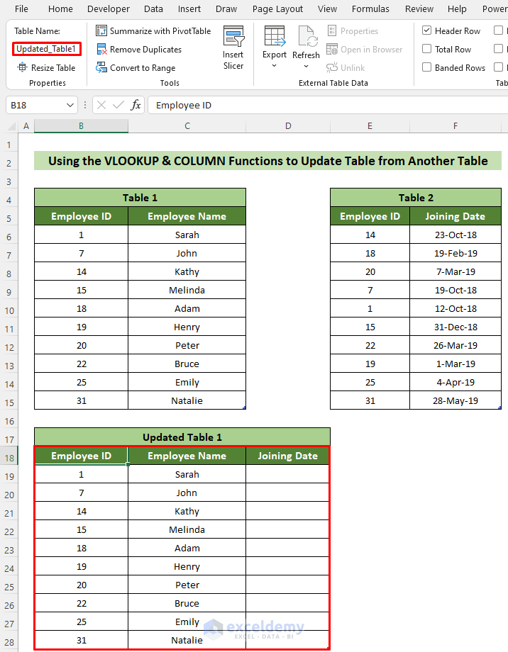
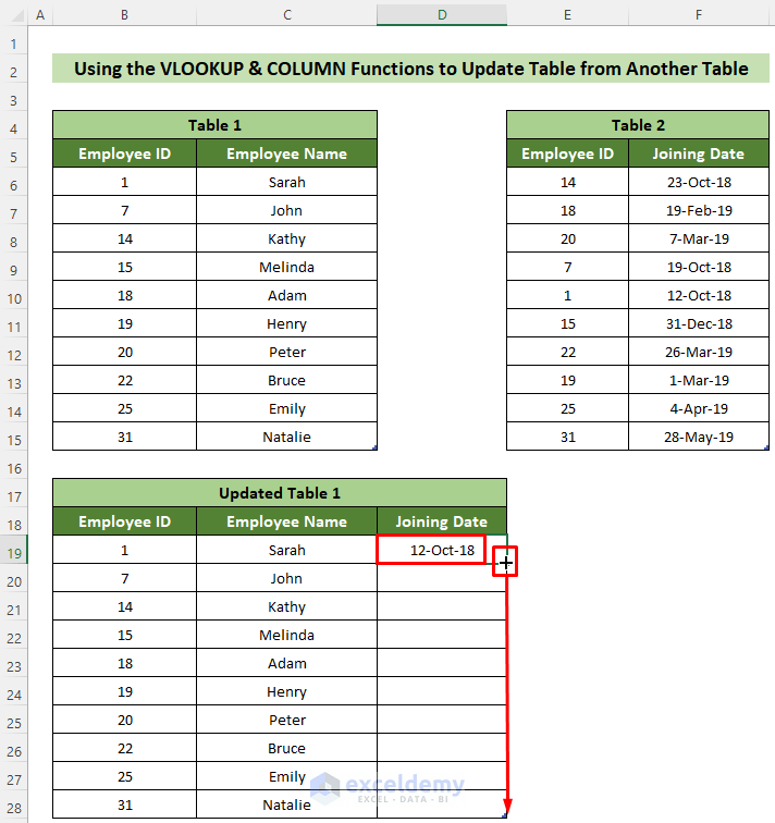
- Create a new table named Updated_Table1 with an additional column for Joining Date.
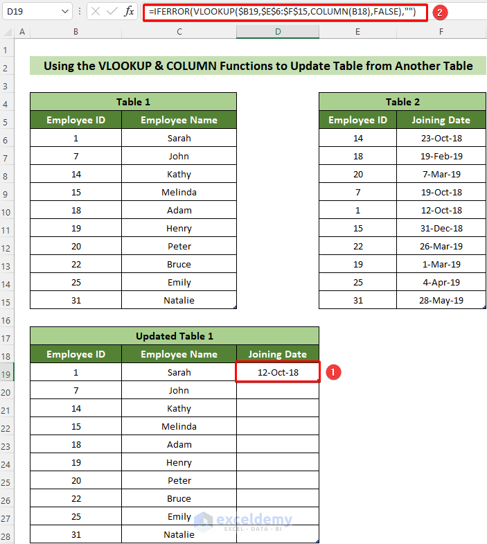
- Click on cell D19 and enter the following formula:
=IFERROR(VLOOKUP($B19,$E$6:$F$15,COLUMN(B18),FALSE),"")-
- This formula retrieves the joining date for Sarah from Table2.
- Press Enter.
- Use the fill handle to copy the formula for the other employees.
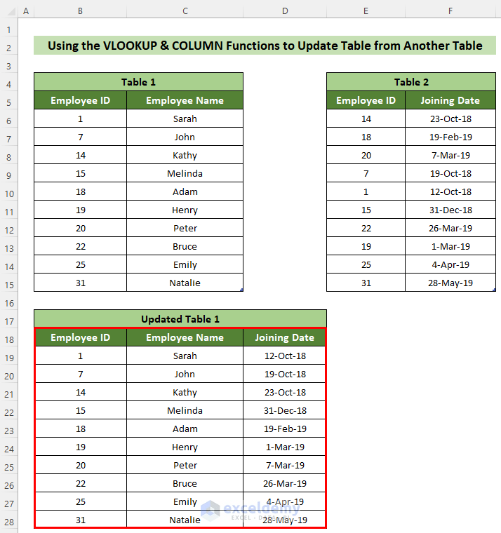
The updated Table1 will now include joining dates based on Employee Name criteria.
Read More: How to Mirror Table on Another Sheet in Excel
Method 3 – Using INDEX and MATCH Functions
We can use INDEX and MATCH functions to update a table from another table.
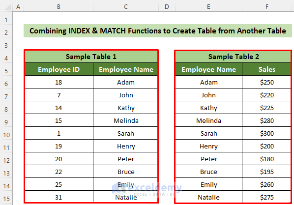
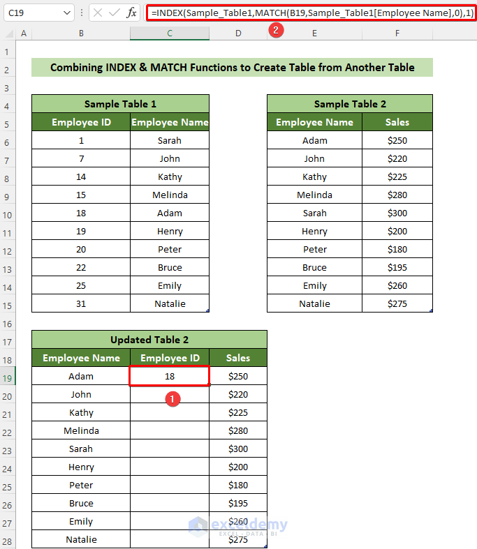
If we are given two tables named Sample_Table 1 and Sample_Table2 and in the first table, there are two columns named Employee ID and Employee Name. The other table contains Employee Name and Sales columns.
We need to insert employee ids in Sample_table2 according to Sample_Table1.
We can achieve this by using the INDEX and MATCH functions.
- Create a new table named Updated_Table2 similar to Sample_Table2 but with an extra column for Employee ID.
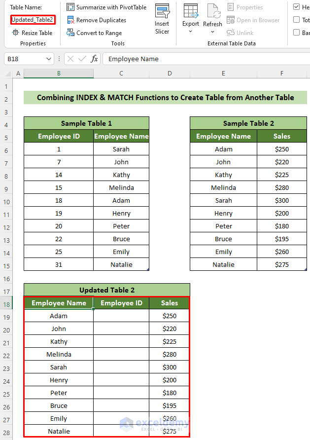
- Click on cell C19 and enter the following formula:
=INDEX(Sample_Table1,MATCH(B19,Sample_Table1[Employee Name],0),1)-
- This formula retrieves the Employee IDs based on their names from Sample_Table1.
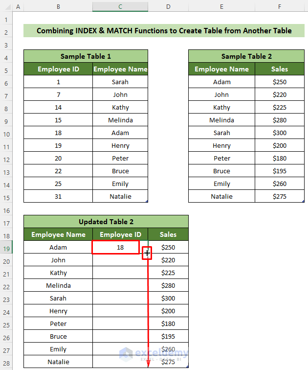
- Press Enter.
- Drag the fill handle downward to complete the Employee IDs for all the names.
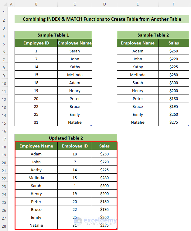
Our updated table will now successfully incorporate Employee IDs based on criteria. The outcome should resemble the provided example.
Read More: How to Create Table from Multiple Sheets in Excel
Download Practice Workbook
You can download the practice workbook from here:
Related Articles
- How to Create a Lookup Table in Excel
- How to Make 3D Table in Excel
- How to Make a Decision Table in Excel
- How to Create a League Table in Excel
- How to Make a Table Bigger in Excel
<< Go Back to Excel Table | Learn Excel
Get FREE Advanced Excel Exercises with Solutions!
