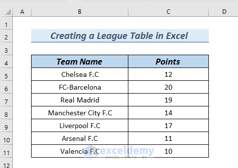
Tocreate a league table in Excel, we’ll use the dataset below, containing some team names and their points totals. We used Microsoft Excel 365 here, but you can use any available Excel version.
Method 1 – Using the RANK Function
Steps:
- Enter the following formula in cell D5:
=RANK(C5,$C$5:$C$11,0)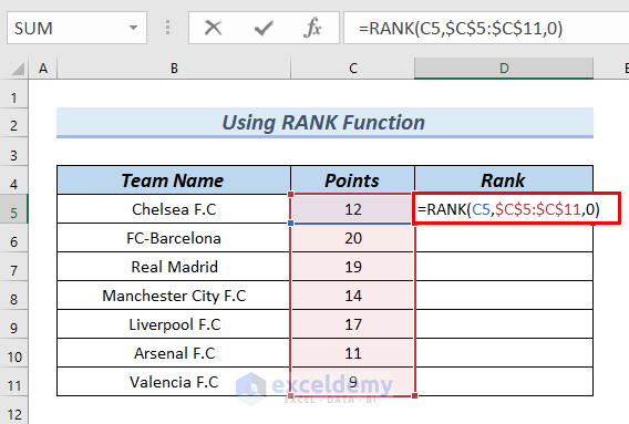
Formula Breakdown
- RANK(C5,$C$5:$C$11,0) → the RANK function returns the rank of a range of numbers.
- C5 → is the number.
- $C$5:$C$11→ is the reference.
- 0 → indicates descending order.
- RANK(C5,$C$5:$C$11,0) → becomes
- Output: 5
- Explanation: Chelsea F.C is at rank 5.
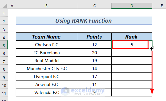
- Press ENTER.
You can see the result in cell D5.
- Drag down the formula with the Fill Handle tool.
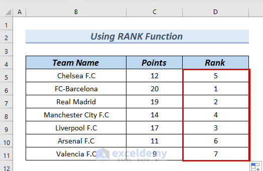
Here is the complete Rank column.
Read More: How to Make a Table Bigger in Excel
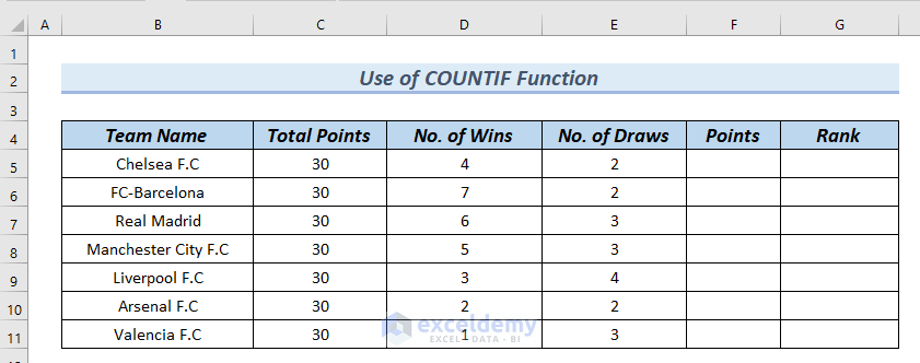
Method 2 – Using the COUNTIF Function
In the following dataset, we have the Team Name, Total Points, No. of Wins, No. of Draws, Points, and Rank columns. First, we will calculate the Points column. Then, using the COUNTIF function, we will determine the Rank column.
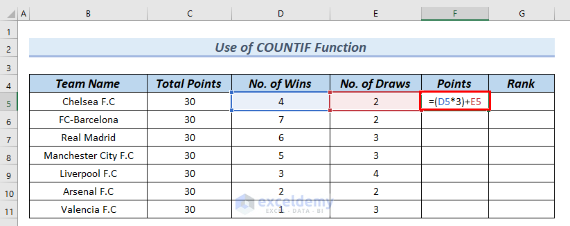
Step 1 – Calculating the Points Column
Teams receive 3 points for each win and 1 point for each draw.
- Enter the following formula in cell F5:
=(D5*3)+E5This simply multiplies the No. of Wins in cell D5 by 3 then adds the No. of Draws in cell E5.
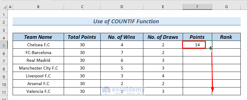
- Press ENTER.
You can see the result in cell F5.
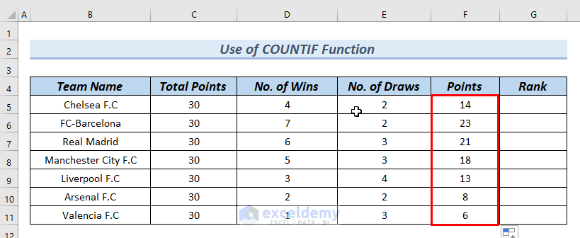
- Drag down the formula with the Fill Handle tool.
As a result, we have the complete Points column.
Step 2 – Ranking the Teams
We will use the COUNTIF function to determine the Rank of the Teams based on their Points totals.
- Enter the following formula in cell G5:
=COUNTIF($F$5:$F$11,">"&F5)+1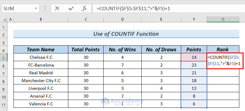
Formula Breakdown
- COUNTIF($F$5:$F$11,”>”&F5)+1 → counts the cells that meet a certain criterion.
- $F$5:$F$11 → is the range of cells
- “>”&F5 → is the criterion.
- +1 → adds 1 to the returned result.
- COUNTIF($F$5:$F$11,”>”&F5)+1→ becomes
- Output: 4
- Explanation: 4 is the rank of team Chelsea F.C.
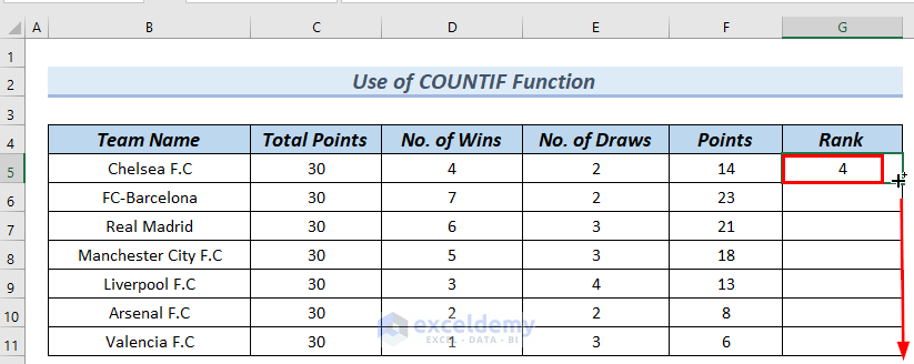
- Press ENTER.
You can see the result in cell G5.
- Drag down the formula with the Fill Handle tool.
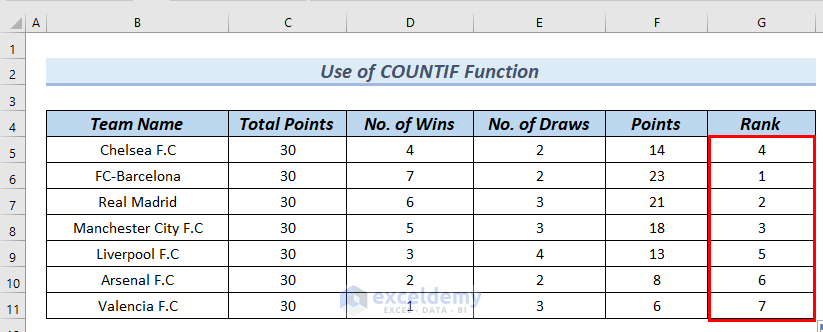
The complete Rank column is filled.
Read More: How to Make a Decision Table in Excel
Method 3 – Using the MATCH and OFFSET Functions to Order Rankings
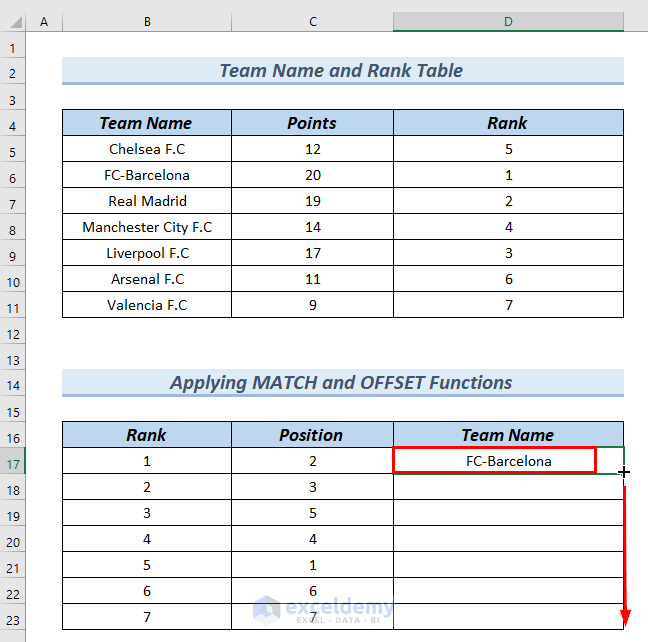
Here, we have an unordered Rank Table. Let’s use the MATCH and OFFSET functions to arrange the teams by Rank.
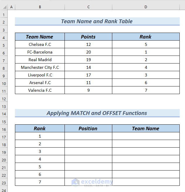
Step 1 – Using the MATCH Function to Get the Position Column
- Enter the following formula in cell C17:
=MATCH(B17,$D$5:$D$11,0)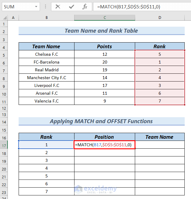
Formula Breakdown
- MATCH(B17,$D$5:$D$11,0) → searches for a specified value in a range of cells.
- B17 → is the lookup_value.
- $D$5:$D$11 → is the lookup_array.
- 0 →indicates an exact match.
- MATCH(B17,$D$5:$D$11,0) → becomes
- Output: 2
- Explanation: 2 is the position of Rank 1 in the Team Name and Rank Table.
- Press ENTER.
You can see the result in cell C17.
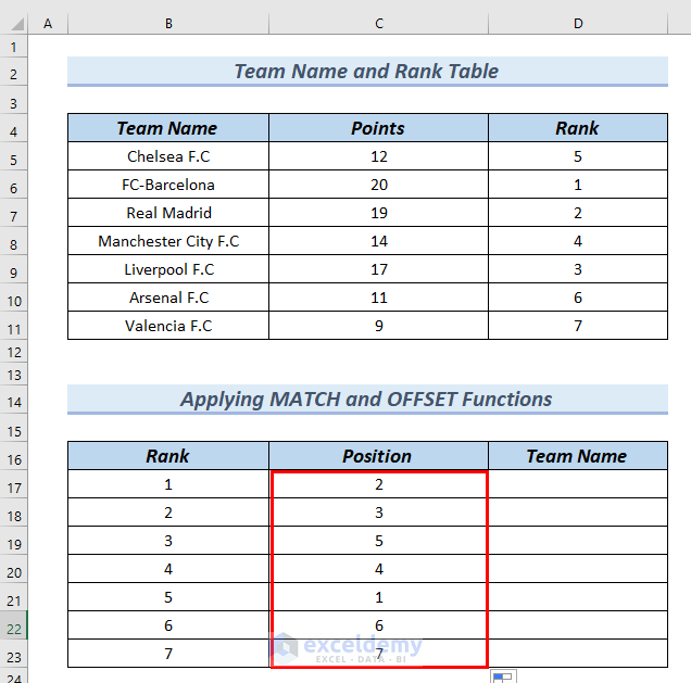
- Drag down the formula with the Fill Handle tool.
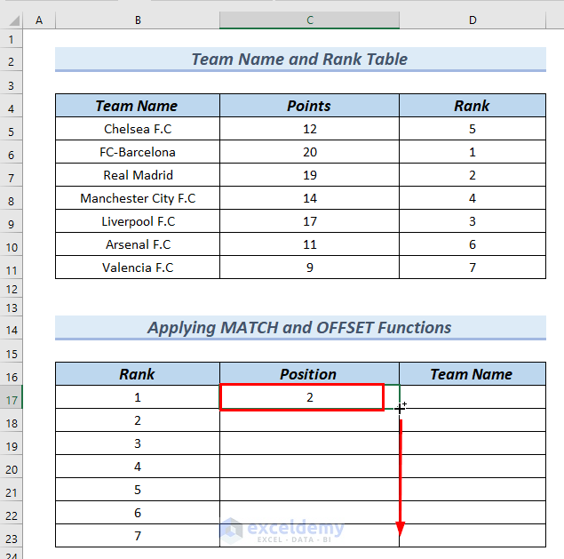
The Position column is filled completely.
Step 2 – Using the OFFSET Function to Find Team Names
- Enter the following formula in cell D17:
=OFFSET($B$4,C17,0) 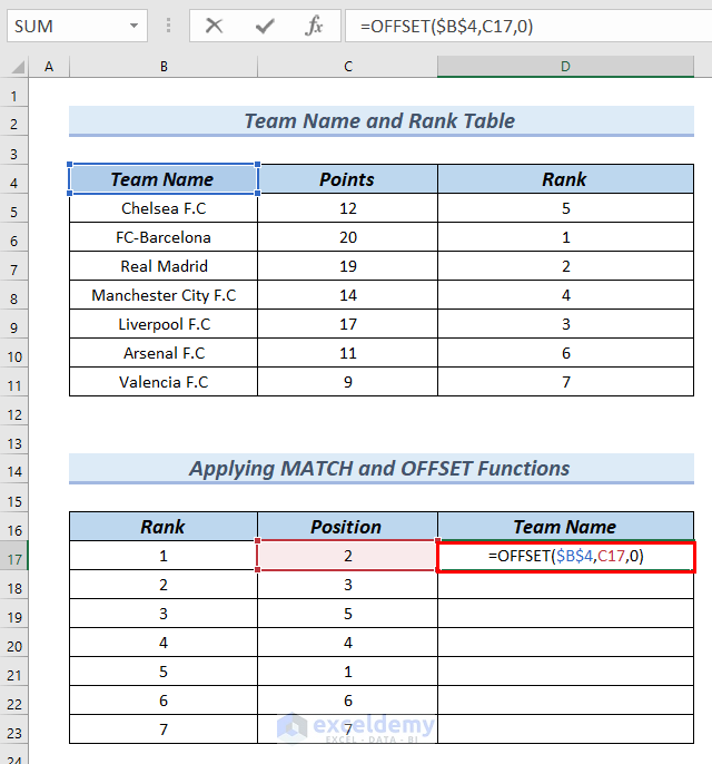
Formula Breakdown
- OFFSET($B$4,C17,0) → returns a part of a dataset with a specific height and width, situated at a specific number of rows down and a specific number of columns right from a given cell reference.
- $B$4 → is the reference.
- C17→ is the row.
- 0 → is the column.
- OFFSET($B$4,C17,0) → becomes
- Output: FC-Barcelona
- Explanation: FC-Barcelona is the Team Name for Rank 1.
- Press ENTER.
You can see the result in cell C17.
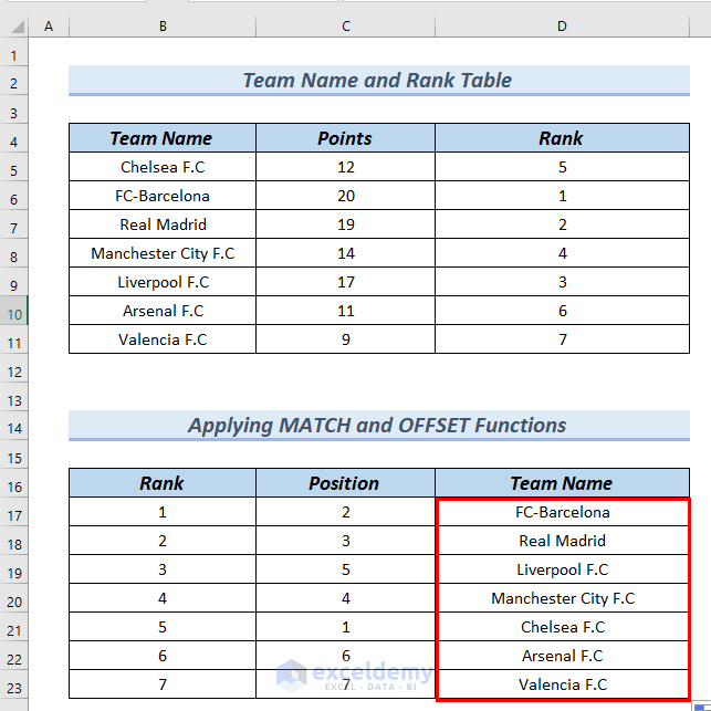
- Drag down the formula with the Fill Handle tool.
We have a league table with the teams ranked in the correct order with the correct Team Names.
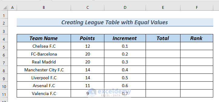
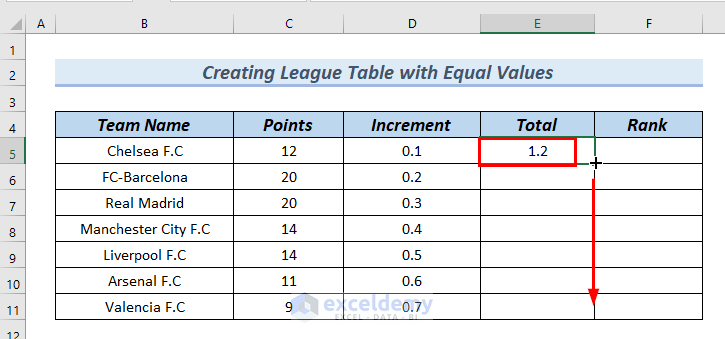
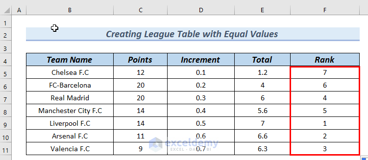
Method 4 – Creating a League Table with Equal Values
In the following dataset, cells C6, and C7 have equal Points, as so cells C8, and C9. Let’s rank our teams despite some of them having equal Points.
We added an Increment column to our dataset.
Steps:
- Enter the following formula in cell E5:
=C5*D5This simply multiplies Points by Increment to get the Total.
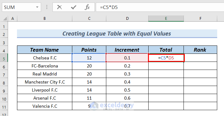
- Press ENTER.
You can see the result in cell E5.
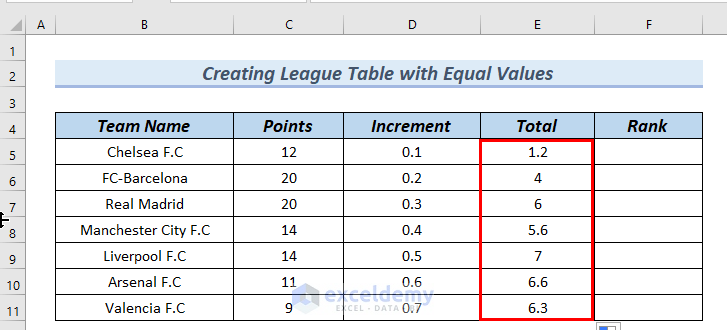
- Drag down the formula with the Fill Handle tool.
The Total column is filled.
Now no teams have equal points, so we can rank them according to their Total.
- Enter the following formula in cell F5:
=RANK(E5,$E$5:$E$11,0)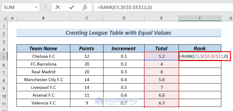
Formula Breakdown
- RANK(E5,$E$5:$E$11,0) → the RANK function returns the rank of a range of numbers.
- E5 → is the number.
- $E$5:$E$11→ is the reference.
- 0 → indicates descending order.
- RANK(E5,$E$5:$E$11,0) → becomes
- Output: 7
- Explanation: Chelsea F.C is at rank 7.
- Press ENTER.
You can see the result in cell D5.
- Drag down the formula with the Fill Handle tool.
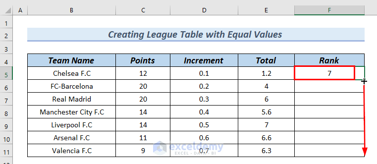
The Rank column is complete.
How to Create League Table with Auto Sorting
The Data Set below is unsorted. Let’s auto-sort it using the SORT function.
The SORT function is only available in Excel 365 or later versions of Excel.
Steps:
- Enter the following formula in cell B17:
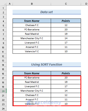
=SORT(B5:C11,2,-1)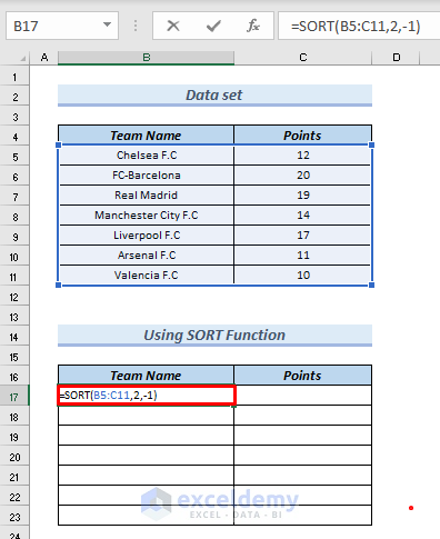
Formula Breakdown
- SORT(B5:C11,2,-1) →The SORT function sorts a range of cells according to a specified sort_index and order.
- B5:C11 → is the table_array.
- 2 → is the sort_index.
- -1 → indicates ascending order.
- Press ENTER.
The sorted league table is returned.
Download Practice Workbook
Related Articles
- How to Create Table from Another Table in Excel
- How to Create Table from Another Table with Criteria in Excel
- How to Mirror Table on Another Sheet in Excel
- How to Create Table from Multiple Sheets in Excel
- How to Create a Lookup Table in Excel
- How to Make 3D Table in Excel
<< Go Back to Excel Table | Learn Excel
Get FREE Advanced Excel Exercises with Solutions!
