Introduction to Excel OFFSET Function
The OFFSET function allows you to start from a specific cell reference, move a certain number of rows down, then a specific number of columns right, and finally extract a section of data with a specific height and width.
Note: The OFFSET function is an array function. To use it, press Ctrl + Shift + Enter unless you’re using Office 365.
Syntax
The syntax for the OFFSET function is as follows:
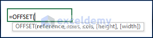
=OFFSET(reference,rows,cols,[height],[width])Arguments
| Arguments | Required or Optional | Value |
|---|---|---|
| reference | Required | The cell reference from which the movement starts. |
| rows | Required | The number of rows to move downward. |
| cols | Required | The number of columns to move rightward. |
| [height] | Optional | The number of rows in the extracted data section (default is 1). |
| [width] | Optional | The number of columns in the extracted data section (default is 1). |
Return Value
- The OFFSET function returns a section of data with the specified height and width. It is located a specific number of rows down and a specific number of columns right from the given cell reference.
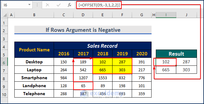
- If the rows argument is negative, the function moves upward from the reference cell.
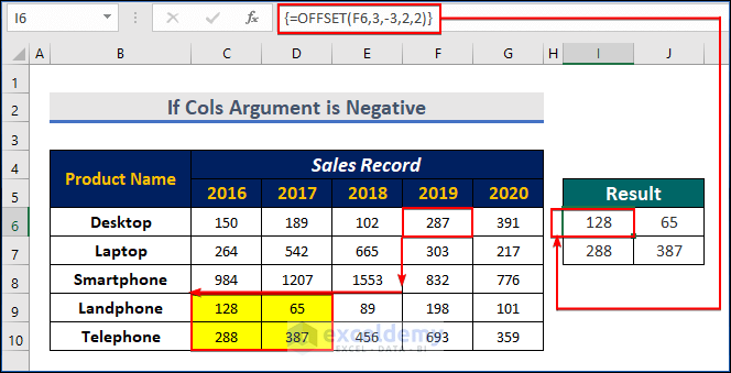
- If the cols argument is negative, the function moves leftward from the reference cell.
Examples
Let’s consider the formula: OFFSET(D9, -3, 1, 2, 2):
- It starts from cell D9.
- Moves 3 rows upward.
- Moves 1 column rightward.
- Collects a section of 2 rows height and 2 columns width.
Similarly, OFFSET(F6, 3, -3, 2, 2) starts from cell F6, moves 3 rows downward, 3 columns leftward, and collects a 2×2 section.
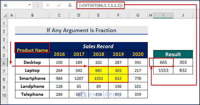
- If any of the arguments (rows, cols, [height], or [width]) is a fraction, Excel automatically converts it to an integer.
In the formula OFFSET(B4,3.7,3,2,2):
- The row argument is a fraction, 3.7.
- Excel has converted it to 3 and then moved 3 rows down from B4 and then 3 columns right.
- And then collected a section of 2 rows high and 2 columns wide.
Method 1 – Extracting a Whole Row
In this method, we’ll use the OFFSET function to extract all values for a whole row. Let’s say we have a sales record spanning 5 years for 13 products from the company Mars Group. To extract the sales record for Television across all years:
- Television is the 7th product on the list.
- The data section spans 5 years (5 columns).
The formula would be:
=OFFSET(B5,7,1,1,5)- Remember to press CTRL+SHIFT+ENTER after entering the formula.
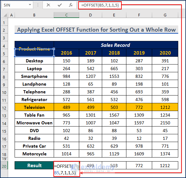
- Start from cell B5.
- Move 7 rows downward to find Television.
- Move 1 column rightward to reach the first year (2016).
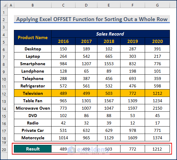
- Extract a section of 1 row height and 5 columns width, representing the sales record of television from 2016 to 2020.
- You’ll see the sales record for Television across all years.
Method 2 – Sorting Out a Whole Column by Using the OFFSET Function in Excel
- Select a whole column from your dataset.
- Let’s find out the sales for the year 2018.
- Note that 2018 corresponds to the 3rd year in our data.
- We want to extract a list of 13 values.
- Enter the following formula:
=OFFSET(B5,1,3,13,1)- Press CTRL+SHIFT+ENTER after entering the formula.
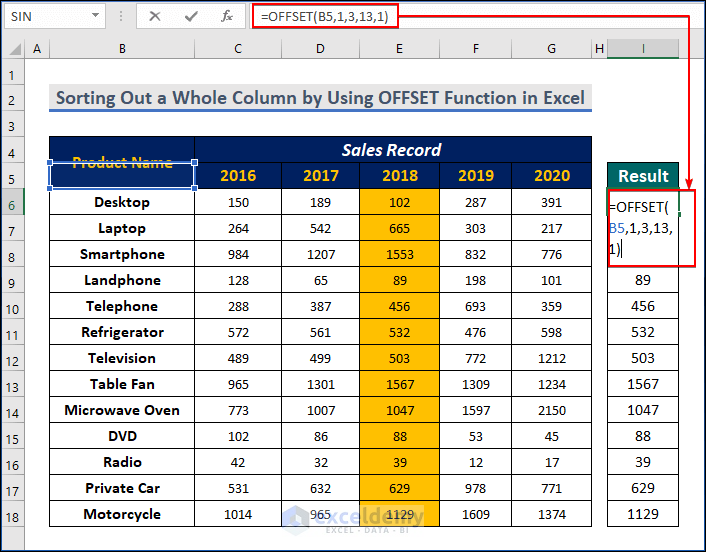
- Begin from cell B5.
- Move 1 row down to the first product (laptop).
- Move 3 columns right to reach the year 2018.
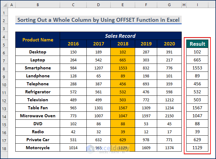
- Extract a section of 13 rows (all products) and 1 column (sales for 2018).
- You’ll see the differentiated sales for the year 2018.
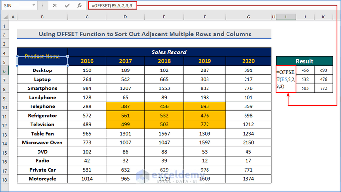
Method 3 – Using the OFFSET Function for Adjacent Multiple Rows and Columns
- Collect a section of multiple rows and columns from your dataset.
- Let’s extract the sales data for the products telephone, refrigerator, and television in the years 2017, 2018, and 2019.
- Telephone is the 5th product on the list.
- 2017 corresponds to the 2nd year.
- Enter the following formula:
=OFFSET(B4,5,2,3,3)- Press CTRL+SHIFT+ENTER after entering the formula.
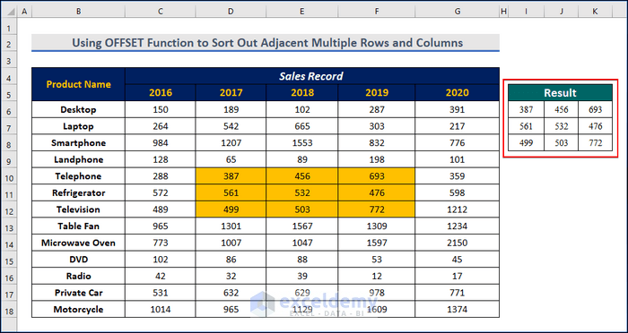
- Start from cell B5.
- Move 5 rows down to the product telephone.
- Move 2 columns right to reach the year 2017.
- Collect data from 3 rows (Telephone, Refrigerator, and Television) and 3 columns (2017, 2018, and 2019).
- You’ve now collected the sales records for Telephone, Refrigerators, and Televisions from 2017 to 2019.
- Remember that the #VALUE error occurs when any argument is of the wrong data type. For example, if the row argument is text instead of a number, it will display #VALUE.
Download Practice Workbook
You can download the practice workbook from here:
<< Go Back to Excel Functions | Learn Excel
Get FREE Advanced Excel Exercises with Solutions!
